Calibration of the Highway Safety Manual and Development of New Safety Performance Functions for Rural Multilane Highways in Kansas

Transcription

1 Report No. K-TRAN: KSU-14-3 FINAL REPORT October 2016 Calibration of the Highway Safety Manual and Development of New Safety Performance Functions for Rural Multilane Highways in Kansas Sunanda Dissanayake, Ph.D., P.E. Syeda Rubaiyat Aziz Kansas State University Transportation Center

2

3 1 Report No. 2 Government Accession No. 3 Recipient Catalog No. K-TRAN: KSU Title and Subtitle 5 Report Date Calibration of the Highway Safety Manual and Development of New Safety October 2016 Performance Functions for Rural Multilane Highways in Kansas 6 Performing Organization Code 7 Author(s) Sunanda Dissanayake, Ph.D., P.E., Syeda Rubaiyat Aziz 7 Performing Organization Report No. 9 Performing Organization Name and Address Kansas State University Transportation Center Department of Civil Engineering 2128 Fiedler Hall Manhattan, KS Sponsoring Agency Name and Address Kansas Department of Transportation Bureau of Research 2300 SW Van Buren Topeka, Kansas Supplementary Notes For more information write to address in block Work Unit No. (TRAIS) 11 Contract or Grant No. C Type of Report and Period Covered Final Report December 2013 May Sponsoring Agency Code RE Rural roads account for 90.3% of the 140,476 total centerline miles of roadways in Kansas. In recent years, rural fatal crashes have accounted for about 66% of all fatal crashes. The Highway Safety Manual (HSM) provides models and methodologies for analyzing the safety of various types of highways. Predictive methods in the HSM were developed based on national trends and data from sample states throughout the United States. However, these methodologies are of limited use if they are not calibrated for individual jurisdictions or local conditions. The objective of this study was to analyze the HSM calibration procedures for rural multilane segments and intersections in Kansas. The HSM categorizes rural multilane segments as four-lane divided (4D) and four-lane undivided (4U) segments, and rural multilane intersections as three-legged intersections with minor-road stop control (3ST), fourlegged intersections with minor-road stop control (4ST), and four-legged signalized intersections (4SG). The number of predicted crashes at each segment was obtained according to the HSM calibration process. Results from calibration of rural segments indicated that the HSM overpredicts fatal and injury crashes by 50% and 65% and underpredicts total crashes by 48% and 64% on rural 4D and 4U segments, respectively. The HSM-given safety performance function (SPF) regression coefficients were then modified to capture variation in crash prediction. The adjusted models for 4D and 4U multilane segments indicated significant improvement in crash prediction for rural Kansas. Furthermore, Kansas-specific safety performance functions were developed following the HSM recommendations. In order to develop Kansas-specific SPFs, Negative Binomial regression was applied to obtain the most suitable model. Several additional variables were considered and tested in the new SPFs, followed by model validation on various sets of locations. The Kansas-specific SPFs are capable of more accurately predicting total as well as fatal and injury crashes on multilane segments compared to the HSM and the modified HSM models. In addition to multilane segments, rural intersections on multilane highways were also calibrated according to the HSM methodology. Using crash modification factors for corresponding variables, SPFs were adjusted to obtain final predicted crash frequency at intersections. Obtained calibration factors indicated that the HSM is capable of predicting crashes at intersections on rural multilane sections at satisfactory levels. Findings of this study can be used for improving safety of rural multilane highways in the state of Kansas. 17 Key Words Highway Safety Manual, Safety Performance Functions, Crash Prediction, Rural Multilane Highways 19 Security Classification (of this report) Unclassified Form DOT F (8-72) 20 Security Classification (of this page) Unclassified 18 Distribution Statement No restrictions. This document is available to the public through the National Technical Information Service 21 No. of pages 22 Price 126 i

4 This page intentionally left blank. ii

5 Calibration of the Highway Safety Manual and Development of New Safety Performance Functions for Rural Multilane Highways in Kansas Final Report Prepared by Sunanda Dissanayake, Ph.D., P.E. Syeda Rubaiyat Aziz Kansas State University Transportation Center A Report on Research Sponsored by THE KANSAS DEPARTMENT OF TRANSPORTATION TOPEKA, KANSAS and KANSAS STATE UNIVERSITY TRANSPORTATION CENTER MANHATTAN, KANSAS October 2016 Copyright 2016, Kansas Department of Transportation iii

6 PREFACE The Kansas Department of Transportation s (KDOT) Kansas Transportation Research and New- Developments (K-TRAN) Research Program funded this research project. It is an ongoing, cooperative and comprehensive research program addressing transportation needs of the state of Kansas utilizing academic and research resources from KDOT, Kansas State University and the University of Kansas. Transportation professionals in KDOT and the universities jointly develop the projects included in the research program. NOTICE The authors and the state of Kansas do not endorse products or manufacturers. Trade and manufacturers names appear herein solely because they are considered essential to the object of this report. This information is available in alternative accessible formats. To obtain an alternative format, contact the Office of Public Affairs, Kansas Department of Transportation, 700 SW Harrison, 2 nd Floor West Wing, Topeka, Kansas or phone (785) (Voice) (TDD). DISCLAIMER The contents of this report reflect the views of the authors who are responsible for the facts and accuracy of the data presented herein. The contents do not necessarily reflect the views or the policies of the state of Kansas. This report does not constitute a standard, specification or regulation. iv

7 Abstract Rural roads account for 90.3% of the 140,476 total centerline miles of roadways in Kansas. In recent years, rural fatal crashes have accounted for about 66% of all fatal crashes. The Highway Safety Manual (HSM) provides models and methodologies for analyzing the safety of various types of highways. Predictive methods in the HSM were developed based on national trends and data from sample states throughout the United States. However, these methodologies are of limited use if they are not calibrated for individual jurisdictions or local conditions. The objective of this study was to analyze the HSM calibration procedures for rural multilane segments and intersections in Kansas. The HSM categorizes rural multilane segments as four-lane divided (4D) and four-lane undivided (4U) segments, and rural multilane intersections as three-legged intersections with minor-road stop control (3ST), four-legged intersections with minor-road stop control (4ST), and four-legged signalized intersections (4SG). The number of predicted crashes at each segment was obtained according to the HSM calibration process. Results from calibration of rural segments indicated that the HSM overpredicts fatal and injury crashes by 50% and 65% and underpredicts total crashes by 48% and 64% on rural 4D and 4U segments, respectively. The HSM-given safety performance function (SPF) regression coefficients were then modified to capture variation in crash prediction. The adjusted models for 4D and 4U multilane segments indicated significant improvement in crash prediction for rural Kansas. Furthermore, Kansas-specific safety performance functions were developed following the HSM recommendations. In order to develop Kansas-specific SPFs, Negative Binomial regression was applied to obtain the most suitable model. Several additional variables were considered and tested in the new SPFs, followed by model validation on various sets of locations. The Kansasspecific SPFs are capable of more accurately predicting total as well as fatal and injury crashes on multilane segments compared to the HSM and the modified HSM models. In addition to multilane segments, rural intersections on multilane highways were also calibrated according to the HSM methodology. Using crash modification factors for corresponding variables, SPFs were adjusted to obtain final predicted crash frequency at intersections. Obtained calibration factors indicated that the HSM is capable of predicting crashes at intersections on rural multilane sections at satisfactory levels. Findings of this study can be used for improving safety of rural multilane highways in the state of Kansas. v

8 Acknowledgements The authors would like to sincerely appreciate the Kansas Department of Transportation (KDOT) for funding this research. Moreover, the authors gratefully thank Ms. Elsit Mandal, Mr. Rex McCommon, and the late Mr. Leif Holliday for their constant support with providing data to complete this research. Appreciations are also extended to the current Project Monitor, Mr. Ben Ware, and previous Project Monitors, Ms. Cheryl Bornheimer and Mr. Howard Lubliner, for their input and support. Assistance provided by State Safety Engineer Mr. Steven Buckley throughout the entire duration of the project is also greatly appreciated. In addition, special thanks extend to Austin Jueneman for assisting with intersection data extraction. vi

9 Table of Contents Abstract... v Acknowledgements... vi Table of Contents... vii List of Tables... ix List of Figures... xi Chapter 1: Introduction Background Highway Safety Manual Problem Statement Objectives of the Study Organization of the Report... 3 Chapter 2: Literature Review Highway Safety Manual Calibration Calibration of Rural Two-Lane Two-Way Highways Calibration of Rural Multilane Highways Development of State-Specific Safety Performance Functions Crash Prediction Studies in Kansas Sample Size for Calibration Process Interactive Highway Safety Design Model SafetyAnalyst Prediction Models Chapter 3: Data and Methodology Data Kansas Crash Analysis and Reporting System Database Control Section Analysis System Google Maps Study Segments Highway Safety Manual Calibration Procedures for Segments Safety Performance Functions Crash Modification Factors Calibration Factor SPF Development Poisson Regression Model vii

10 3.4.2 Negative Binomial Regression Model Model Validation Statistics Intersection Data Highway Safety Manual Calibration Procedures for Intersections Chapter 4: Calibration of HSM Predictive Methods Distribution and Comparison of Crashes Collision Type Severity Level Nighttime Crash Proportions Calibration of Rural Multilane Segments Modification of HSM-Given SPF Calibration of Rural Multilane Intersections Chapter 5: Development of Kansas-Specific New Safety Performance Functions for Rural Four- Lane Divided Segments Model Selection for Kansas-Specific SPFs Highway Segments for New SPF Development New Variables Considered in Kansas-Specific SPFs Horizontal Alignment Vertical Grade Roadside Hazard Rating Speed Limit Driveway Density Correlation Test New SPFs Total Crashes Fatal and Injury Crashes Validation Total Crashes Fatal and Injury Crashes Comparison of New SPF to HSM-given SPF Chapter 6: Summary, Conclusions, and Recommendations Summary and Conclusions Recommendations and Future Work References Appendix: Calibration Data viii

11 List of Tables Table 3.1: Data Sources for Rural Four-Lane Segments Table 4.1: Percentage of Crashes by Collision Type for Kansas Rural Four-Lane Highways Table 4.2: Crash Severity Level on Four-Lane Highways Table 4.3: Crashes by Collision Type and Severity Level for Four-Lane Roadways Table 4.4: Crash Distribution by Light Condition Table 4.5: Proportion of Nighttime Crashes for Rural 4D and 4U Highways in Kansas Table 4.6: Descriptive Statistics for Rural Four-Lane Segments Table 4.7: 4D Segments Sample Worksheet Table 4.8: 4D Segments Calibration Factor Calculation Table 4.9: 4U Segments Sample Worksheet Table 4.10: 4U Segments Calibration Factor Calculation Table 4.11: Comparison of Regression Coefficients Table 4.12: New Calibration Factors with the Modified SPF Table 4.13: Descriptive Statistics for Rural Multilane Intersections Table 4.14: 4ST Intersection Sample Worksheet Table 4.15: Calculation of Calibration Factors for 4ST Intersections Table 4.16: 3ST Intersection Sample Worksheet Table 4.17: Calculation of Calibration Factors for 3ST Intersections Table 5.1: Variables in New SPF Development Table 5.2: Curve Classifications Table 5.3: Vertical Grade Classifications Table 5.4: Roadside Hazard Rating Criterion Table 5.5: Descriptive Statistics of Variables Table 5.6: Correlation Analysis of Variables Table 5.7: Parameter Estimates of Model 1 for Predicting Total Crashes Table 5.8: Parameter Estimates of Model 2 for Predicting Total Crashes Table 5.9: Parameter Estimates of Model 3 for Predicting Total Crashes Table 5.10: Parameter Estimates of Model 4 for Predicting Total Crashes Table 5.11: Parameter Estimates of Model 1 for Predicting Fatal and Injury Crashes Table 5.12: Parameter Estimates of Model 2 for Predicting Fatal and Injury Crashes Table 5.13: Parameter Estimates of Model 3 for Predicting Fatal and Injury Crashes ix

12 Table 5.14: Parameter Estimates of Model 4 for Predicting Fatal and Injury Crashes Table 5.15: Goodness-of-Fit Comparison for Total Crashes Model Table 5.16: Goodness-of-Fit Comparison of Fatal and Injury Crash Models Table 5.17: Comparison of Model Statistics Table A.1: List of Locations for 4D Segment Calibration Table A.2: List of Locations for 4U Segment Calibration Table A.3: List of Locations for 4ST Intersections Calibration Table A.4: List of Locations for 3ST Intersections Calibration x

13 List of Figures Figure 1.1: Yearly Distribution of Crashes in Kansas... 2 Figure 3.1: Using Google Map to Obtain Presence of Lighting Figure 3.2: Rural 4D Segments and Crash Location Map Figure 3.3: Rural 4U Segments and Crash Location Map Figure 3.4: 4ST Intersection with Stop Control at Minor Approach Figure 3.5: 3ST Intersection with Stop Control at Minor Approach Figure 3.6: Use of KDOT Videologs Figure 3.7: Intersection-Box Demonstration Figure 4.1: Distribution of Crash Frequency on 4D Segments Figure 4.2: Distribution of Crash Frequency on 4U Segments Figure 4.3: Distribution of Crash Frequency on 4ST Intersections Figure 4.4: Distribution of Crash Frequency on 3ST Intersections Figure 5.1: Total Crashes: Model 1 Validation Plot Figure 5.2: Total Crashes: Model 2 Validation Plot Figure 5.3: Total Crashes: Model 3 Validation Plot Figure 5.4: Total Crashes: Model 4 Validation Plot Figure 5.5: Total Crashes: Model 1 Validation Plot (Without Outliers) Figure 5.6: Total Crashes: Model 2 Validation Plot (Without Outliers) Figure 5.7: Total Crashes: Model 3 Validation Plot (Without Outliers) Figure 5.8: Total Crashes: Model 4 Validation Plot (Without Outliers) Figure 5.9: Fatal and Injury Crashes: Model 1 Validation Plot Figure 5.10: Fatal and Injury Crashes: Model 2 Validation Plot Figure 5.11: Fatal and Injury Crashes: Model 3 Validation Plot Figure 5.12: Fatal and Injury Crashes: Model 4 Validation Plot Figure 5.13: Fatal and Injury Crashes: Model 1 Validation Plot (Without Outliers) Figure 5.14: Fatal and Injury Crashes: Model 2 Validation Plot (Without Outliers) Figure 5.15: Fatal and Injury Crashes: Model 3 Validation Plot (Without Outliers) Figure 5.16: Fatal and Injury Crashes: Model 4 Validation Plot (Without Outliers) xi

14 This page intentionally left blank. xii

15 Chapter 1: Introduction 1.1 Background According to a study published in 2016, motor vehicle crashes were one of the top 10 causes of death in the United States in 2013 (Heron, 2016). Relative to 2011, fatal highway crashes increased by 1.7% to 29,989 in 2014, equivalent to an average of 90 daily fatalities. Despite the decline in fatalities, 32,675 deaths occurred as a result of roadway crashes in the United States in 2014, down from 32,894 in 2013 (NHTSA, 2016). Rural roads account for 90.3% of the 140,476 total miles of roadway in Kansas (KDOT, 2015a), and in 2014, rural travel accounted for 48.5% of all vehicle miles (60% for state highways; KDOT, 2015b). Figure 1.1 shows the distribution of rural, urban, fatal rural, fatal urban, and total crashes over a 14-year period. In general, Kansas has a low population density and a majority of the roadways are in rural areas. As shown in Figure 1.1, 35% of total crashes occurred on rural roads, while fatal crashes on rural roads accounted for over 66% of the number of total fatal crashes in Kansas during 2014 (KDOT, 2015a). This is not only in 2014; every year the number of fatal crashes on rural highways has always been considerably higher than the fatal crashes on urban highways in Kansas. The time required to respond and transport crash victims potentially determines if the crash is classified as injury or fatal. In rural areas, transportation of severely injured crash victims to hospitals requires minutes (NHTSA, 2009). These numbers are a matter of concern for highway safety professionals because they comprise a major proportion of high-level injury crashes in rural areas. 1.2 Highway Safety Manual The Highway Safety Manual (HSM) from the American Association of State Highway and Transportation Officials (AASHTO) is the culmination of decades of safety research and practices. The HSM provides models and methodologies for analyzing various types of highways based on safety. The first version, published in 2010, was updated in 2014 with new chapters on predictive methods for freeways and ramps. Procedures to calibrate predictive models are currently available in Appendix A of Part C in the HSM (AASHTO, 2014). Crash predictive methods in the HSM allow planners, designers, and reviewers to comprehensively assess 1

16 expected safety performance of highway design via methodologies endorsed by the Federal Highway Administration (FHWA). Predictive methods in the HSM were developed based on national trends and statistics from sample states throughout the United States. However, these methodologies are of limited use if they are not calibrated for individual jurisdictions or local conditions. Calibration ensures the most realistic and reliable crash estimates. Number of Crashes 80,000 70,000 60,000 50,000 40,000 30,000 20,000 10, Number of Fatal Crashes Year 0 Total crashes Urban crashes Rural crashes Fatal Rural crashes Fatal Urban crashes Figure 1.1: Yearly Distribution of Crashes in Kansas 1.3 Problem Statement Safety conditions of highways change over time; therefore, agencies should only use the HSM models that have been calibrated. Uncalibrated models compromise safety estimates, produce unrealistic results, and undermine accountability of highway safety. Even agencies that use their own data to develop SPFs should consider calibrating the models every 2 to 3 years in order for results to be comparable to estimates obtained from an agency s records. An acceptable method to predict crashes for rural multilane highway segments and intersections in Kansas must be developed. Currently, the Kansas Department of Transportation (KDOT) can apply the rural two-lane model given in the HSM because a previous study 2

17 calibrated such facilities (Lubliner, 2011). KDOT has occasionally requested analysis of a multilane facility, but it cannot be completed without calibration. An effective equation that predicts the number of crashes along a highway and identifies potential high crash locations would enable design engineers to design safer roads while minimizing the cost if, for example, 8- ft shoulders were determined to be as beneficial as 10-ft shoulders. Although calibration procedures are available in the HSM Appendix A, they must be refined or modified to accommodate data availability and roadway, traffic, and crash characteristics in Kansas. The HSM considers only four-lane highways to be categorized as rural multilane. Therefore, this study was limited to calibrations for rural four-lane divided (4D) and four-lane undivided (4U) highways in Kansas. Similar calibration is required on rural multilane intersections, which has not been performed for Kansas to date. So additionally, the rural multilane intersections will be calibrated in this study. 1.4 Objectives of the Study The objective of this report is to analyze the HSM calibration procedures for rural multilane segment and intersection models for Kansas in which rural multilane segments are categorized as 4D and 4U, and intersections are categorized as three-legged intersections with minor-road stop control (3ST) and four-legged intersections with minor-road stop control (4ST). This study utilized the HSM methodology to calibrate the crash predictive method. Since the HSM methodology cannot accurately predict crashes at rural segments, new Kansas-specific models or SPFs were developed and their performances were compared to the HSM-given SPFs. 1.5 Organization of the Report This report contains six chapters and an appendix. Chapter 1 provides background information regarding the HSM methodology and study objectives. Chapter 2 summarizes past research conducted in similar contexts, and Chapter 3 includes discussion of the methodology and data used in this report. Calibration results obtained using the HSM methodology are presented in Chapter 4. Chapter 5 discusses the development of new SPFs, and Chapter 6 summarizes the study with a discussion of future work. 3

18 Chapter 2: Literature Review This chapter summarizes the review of literature, beginning with initial research reporting the relationship of geometric and surrounding features to crash type, followed by SPFs and the evolution of current crash prediction models (CPMs). Although the literature review does not include all CPM-related research, it summarizes the most critical sources that have led to the development of current prominent methods, including recent research of CPM applications. 2.1 Highway Safety Manual Calibration A limited number of studies have performed and documented the HSM calibration process. Sun, Li, Magri, and Shirazi (2006) performed the first study that calibrated the HSM s CPM for two-lane rural highway segments in Louisiana. The CPM used was nearly identical to the current model given in Chapter 10 in the HSM, with the exception that the HSM had additional crash modification factors (CMFs) for rumble strips, lighting, and automated speed enforcement added after the research by Sun et al. In addition, the calibration procedure recommended in the draft HSM that was applied to the study differed from the procedure published in the HSM. It is because the procedure required stratification of calibration factors based on traffic volume. Calibration factors were then averaged together for application Calibration of Rural Two-Lane Two-Way Highways Srinivasan and Carter (2011) developed SPFs for various types of roadways in North Carolina and illustrated how SPFs can improve the decision-making process. The HSM prediction methods were used to compute the calibration factor for total crashes for each facility type. Using data from the crash-reporting database at the North Carolina Department of Transportation (NCDOT), segments within the influence of at-grade intersections and railroad grade crossings (250 ft on either side of at-grade intersections or railroad grade crossings) were removed. SPFs were estimated for nine crash types identified to be of primary importance to NCDOT. In addition, SPFs for rural two-lane roads were estimated by including site characteristics such as shoulder width/type and terrain. Another SPF was used for network 4

19 screening. Srinivasan and Carter also suggested that NCDOT calibrate SPFs developed in this process and/or develop SPFs using Negative Binomial regression. The study by Sun et al. (2006) utilized the same basic definition for rural two-lane highways in Louisiana, but lack of geometric data required the use of default values for several CMFs, and some data values were not consistent with those experienced in Kansas. Using these data and calibration methodology, a calibration value of 1.63 was determined for the Louisiana highway system. The Louisiana study also validated the CPM using the calibration factor and the Empirical Bayes (EB) procedure. The study demonstrated model accuracy in terms of percent difference between observed and predicted crashes with calibration. Accuracy of the calibrated model without the EB procedure yielded a 5.22% difference. The EB procedure improved model accuracy by 3.06%. Accuracies pertained to the aggregates of all segments modeled in the validation study, but results did not show individual segment accuracy in definable values. Xie, Gladhill, Dixon, and Monsere (2011) calibrated each of the HSM-considered roadway facility types in the Oregon highway system. Using data from 2004 to 2006 for rural, two-lane, two-way roads, the final calibration factor was determined to be 0.74, which they speculated to be under 1.0 due to fewer reported property damage only (PDO) crashes, since those crashes do not have to be reported to authorities in Oregon. Xie et al. also found that data accumulation was time-consuming, evidenced by a gap in their research because they did not validate newly created calibration factors. Although they followed steps given in the HSM, they did not verify accuracy of the calibrated model for crash prediction Calibration of Rural Multilane Highways As suggested by the HSM, only 4D and 4U facilities are categorized as rural multilane. A review of studies focusing on rural multilane highway calibration using the HSM is presented herein. Sun, Magri, Shirazi, Gillella, and Li (2011) calibrated the SPF for rural multilane highway segments, investigated how calibrated models work in network screening, and identified potential application issues. Their paper presented results for segments. Among the 600 miles of rural multilane highways in the Louisiana Department of Transportation and 5

20 Development (LaDOTD) system, some highways were divided into control sections based on highway design features and traffic volumes. All design features and traffic conditions were identical within each control section. Coefficients for basic SPFs were obtained from the HSM, and relevant CMFs were applied to the number of predicted crashes. Obtained calibration parameters indicated that the predicted model from the HSM for rural divided multilane highways underestimated expected crashes. Network screening was performed in conjunction with the Safety Management System introduced in Part B of the HSM. The application indicated that, even without the calibrated safety performance model, commonly used crash frequency methods produce results similar to the results of sophisticated models. However, the same thing cannot be said about crash rate methods. Result comparisons of the four screening measures were similar to sample application results presented at the end of Chapter 11 in the HSM (Sun et al., 2011). Sun, Edara, Brown, Claros, and Nam (2013) divided segments in Missouri based on Annual Average Daily Traffic (AADT), an important input for HSM-given CPMs. Characteristics used to subdivide segments included speed category for urban arterials, median type, effective median width for freeways and rural multilane highways, and horizontal curve radius for rural two-lane highways. After subdivision, some segments were shorter than the desired minimum 0.5 miles for rural segments and 0.25 miles for urban segments. Segments ranged in length between 0.56 and 7.59 miles, with an average length of 2.60 miles. This study considered crash data from 2009 to 2011, and AADT of 2011 was obtained from their database. The total number of vehicle crashes was 715 per year, which significantly exceeded the HSMrecommended 100 crashes per year. A median width of 30 ft was used for segments with a median barrier, as recommended by the HSM. Segment length was calculated as the average segment length in both directions, excluding interchange limits. Results indicated close agreement between the number of crashes predicted by the HSM and the number of crashes observed in Missouri for those site types. Lord et al. (2008) developed a methodology to predict the safety performance of elements in the planning, design, and operation of nonlimited-access rural highways. Models were proposed for the three types of intersections and undivided and divided highway segments by 6

21 crash type and crash severity. They collected data from databases in California, Minnesota, New York, Texas, and Washington, which they used to develop statistical models and CMFs for intersections and segments as well as a cross-validation study to evaluate the recalibration procedure for jurisdictions other than those for which the models were estimated. They utilized data collected in Texas, California, Minnesota, and Washington to develop models and CMFs, and they used New York data for cross-validation. The collected data included detailed information about geometric design characteristics, traffic flow, and motor vehicle crashes. Jalayer, Zhou, Williamson, and LaMondia (2015) presented a revised method to develop calibration factors for five types of urban and suburban roadways with consideration of the recent crash recording threshold (CRT) change, a minimum value to report crashes, in Illinois. Because of a change in 2009 regarding the recording threshold for PDO crashes, the study established a revised method to supplement and adopt a standard approach to develop calibration factors in the HSM, considering impact of the new CRT. The higher the CRT, the fewer recorded PDO crashes. Before and after the threshold change, 4D calibration factors were 0.68 and 0.55, respectively. Because the threshold change only affects the total number of crashes and PDO crashes, percentage distributions of fatal and injury crashes before the threshold change were adjusted in order to accurately estimate the total number of fatal and injury crashes. This study provided a revised method to help state and local agencies predict the number of crashes without redeveloping new calibration factors due to change in CRT. 2.2 Development of State-Specific Safety Performance Functions A unique Oregon study by Xie et al. (2011) developed jurisdiction-specific crash distributions to replace default values in the HSM. Their analysis showed that, on an aggregate level, use of jurisdiction-specific distributions did not significantly affect results compared to HSM default values. However, this analysis did not include quantification of this impact at the project level. Of the statistics provided, Oregon-specific values also did not vary notably from default values in the HSM; therefore, no significant impact was found using Oregon-specific values instead of default values. 7

22 Banihashemi (2011) compared CPM calibration to two new SPFs in the state of Washington. Equation 2.1 has the same general form as the rural two-lane SPF in the HSM, and Equation 2.2 has a similar form except that AADT is raised to the power of Four new statespecific CMFs were produced and used with the new SPFs in this study: lane width, shoulder width, curve radius, and vertical grade. Results showed that calibration in Washington was identical for any of the new models, but the newer models may be preferable if created specifically for Washington. However, because the original SPF was created using data from Washington and Minnesota, this model was expected to work just as well as new SPFs. Similar to previous studies, models studied by Banihashemi assumed default values for a number of CMFs due to data limitations. NN ssppff 1 rrss = AAAADDTT LL Equation 2.1 NN ssppff 2 rrss = AAAADDTT 1.05 LL Equation 2.2 Where: AADT = average annual daily traffic (vpd), and L = length of segment (mi). Qin, Zhi, and Vachal (2014) applied the HSM methodology to rural two-lane, two-way highway segments in South Dakota. Calibration was based on 3 years ( ) of crash data from 657 roadway segments, totaling more than 750 miles of roadways. The calibration process established new base conditions, developed SPFs, converted CMFs to base conditions, and substituted default values with state-specific values. Five models were developed and compared based on statistical goodness-of-fit and calibration factors. Results showed that jurisdictionspecific crash type distribution for CMFs drastically differed from crash distribution presented in the HSM. The HSM method without modification was shown to underestimate crashes in South Dakota by 35%. The method based on SPFs developed from a full model demonstrated the best model fit. This study provided important guidance and empirical results regarding calibration of HSM models. Mehta and Lou (2013) evaluated applicability of the HSM predictive methods on Alabama data for two-lane, two-way rural roads and 4D highways. They calibrated the HSM- 8

23 based SPFs using two approaches, and they proposed a new approach that treats the estimation of calibration factors as Negative Binomial regression. Data was taken from the years of 2006 to In addition, new forms for state-specific SPFs were investigated to identify the best model using Poisson-Gamma regression techniques. Mehta and Lou studied four new model forms and evaluated prediction capabilities of the two calibrated models and four newly developed statespecific SPFs using a validation data set. They considered five performance measures for model evaluation: mean absolute deviance, mean squared prediction error, mean prediction bias, log likelihood value, and Akaike information criterion (AIC). The study identified a state-specific SPF that accurately fit the Alabama data and outperformed other models, including calibrated SPFs. The best model described mean crash frequency as a function of AADT, segment length, lane width, year, and speed limit. Results showed that the HSM-recommended method for calibration factor estimation performed well, proving to be a straightforward, easily applicable approach even though it was not as good as the best state-specific SPF. 2.3 Crash Prediction Studies in Kansas Similar to other transportation organizations, KDOT has researched more efficient ways to screen robust system inventories and crash data in order to identify relationships between highway features and safety. Najjar and Mandavilli (2009) used artificial neural networks (ANNs) to attempt to identify these relationships for Kansas highways. Their research included the six major types of roadway networks in Kansas: rural Kansas Turnpike Authority (KTA), rural two-lane, rural expressway, rural freeway, urban freeway, and urban expressway. The models evaluated total crash rate as well as fatal, injury, and severe injury crash rates. For rural two-lane highways, Najjar and Mandavilli identified eight variables that affect crashes: Section length Surface width Route class Shoulder width (outside) Shoulder type (outside) AADT Average percentage of heavy trucks Average speed limit 9

24 ANN models produced by Najjar and Mandavilli (2009) were measured against training, testing, and validation data sets. The overall rural two-lane model produced an R 2 of The total crash rate model was most similar to the HSM model in this research; the R 2 value for the total crash rate ANN model was Lubliner and Schrock (2012) analyzed multiple predictive methods to calibrate rural twolane segment SPFs in Kansas. They initially analyzed all methods published in the HSM to determine method accuracy. Calibrated predictions showed significant improvements compared to uncalibrated predictions, and they were extremely accurate when analyzed at the aggregate level. In order to improve crash prediction accuracy, Lubliner and Schrock analyzed alternative calibration methods, including linear calibration methods that address variables previously shown to positively correlate to highway crashes in Kansas but are not considered in the HSM. Although linear calibration methods did not perform as well on the aggregate level, they were more accurate on the project level. In general, analysis of the HSM rural two-lane segment predictions showed favorable accuracy, leading to recommended inclusion in KDOT s safety evaluation toolbox at the project level. Based on study results, single statewide calibration of total crashes was recommended for aggregate analyses that include multiple sections. However, the study by Lubliner and Schrock contained a large proportion of animal-related crashes, totaling 58.9% of animal-related crashes in Kansas but only 12.1% animal-related crashes in the HSM crash distribution. Therefore, an additional obtained calibration factor considered only crashes without animals, resulting in a calibration value of Final calibrations considered animal crash rates of each segment and county, with the county, or variable, calibration factor working best according to: CC ccoouunnttyy = 1.13 AACCRR ccoouunnttyy Equation 2.3 Where: CC cc oo uu nn tt yy = calibration factor for a county, and AA CC RR cc oo uu nn tt yy = deer crash rate for a county. 10

25 Results showed that CC cc oo uu nn tt yy worked best, but they suggested additional research to create a jurisdiction-specific SPF in order to determine if it could more accurately predict crashes on rural Kansas highways compared to the HSM model calibration (Lubliner & Schrock, 2012). Bornheimer (2011) tested the original HSM CPMs to state-specific calibrated CPMs and new, independent CPMs to determine the best model for rural two-lane highways in Kansas. They collected nearly 300 miles of highway geometric data to create the new models using Negative Binomial regression. The most significant variables in each model were consistently lane width and roadside hazard rating. These models were compared to CPMs calibrated for the HSM using nine validation segments. However, one comparison difficulty was the large amount of animal-related crashes, accounting for 58.9% of crashes on Kansas highways. Analysis results showed that two models work best for Kansas: the variable calibration method in which crashes are predicted using the HSM s CPM and a calibration based on animal crash rates by county that demonstrates high correlation using Pearson s R. The variable calibration method also considers individual county animal crash statistics, thereby accounting for animal crashes. The model was run using the HSM s CPM method and the Interactive Highway Safety Design Model (IHSDM), requiring in-depth data mining to collect all variables. Equation 2.4 defines the calibration factor, CC cc oo uu nn tt yy, used in the HSM equation, as shown in Equation 2.5. CC ccoouunnttyy = 1.13 AACCRR ccoouunnttyy Equation 2.4 NN pprreeddiicctteedd rrss = NN ssppff rrss (CCMMFF 1rr CCMMFF 2rr CCMMFF 12rr) Equation 2.5 The non-animal model, restated in Equation 2.6, is a new SPF created using only crashes that did not involve an animal. This model had high correlation and low Bayesian Information Criterion (BIC), making it a good candidate. Elimination of animal-related crashes, which were generally out of an engineer s control, improved SPF. The SPF shown in Equation 2.6 also requires roadside hazard rating (RHR), AADT, and length of segment (L), thereby reducing the number of required variables and resulting in less effort to collect data during application (Bornheimer, 2011). 11

26 NN pprreedd nnoo aann = AAAADDTT 1.01 LL 0.85 ee ( RRHHRR ) Equation 2.6 Where: AADT = average annual daily traffic (vpd), and L = length of segment (mi). 2.4 Sample Size for Calibration Process Sample size significance and influence also extensively influence the calibration process. Shin, Lee, and Dadvar (2014) completed the calibration process for SPFs in the HSM for the Maryland Department of Transportation (MDOT) in order to determine a statistically reliable sample size for developing local calibration factors (LCFs) and calculating the confidence interval for the range of calibration factors containing 90% of the population. Study results showed that calibration factor ranges were wider for site types with small populations. Another study used data from the state of Washington to determine the ideal sample size for calibrating the HSM models and to examine sensitivity in a variety of HSM calibration factor sample sizes in order to evaluate the quality of developed factors (Banihashemi, 2012). Roadway and crash data were obtained for a 3-year period ( ). Calibration factors generated from the entire data set for each highway type were considered ideal calibration factors, and factors generated from various data set sizes were compared to the ideal factors. The probability that generated calibration factors fell within 5% and 10% of the ideal calibration factor was calculated. Results of this sensitivity analysis were reviewed and recommendations were derived and presented (Banihashemi, 2012). 2.5 Interactive Highway Safety Design Model The IHSDM is a suite of software analysis tools used to evaluate the safety and operational effects of geometric design on highways. The IHSDM is a decision-support tool that estimates a highway design s expected safety and operational performance and compares existing or proposed highway designs to relevant design policy values. Results of the IHSDM support decision making in the highway design process. Intended users include highway project managers, designers, and traffic and safety reviewers in state and local highway agencies and engineering consulting firms. The IHSDM, which supports the data-driven safety analysis 12

27 initiative of the FHWA s Every Day Counts Round 3 (EDC-3) efforts, includes six evaluation modules: Crash Prediction, Design Consistency, Intersection Review, Policy Review, Traffic Analysis, and Driver/Vehicle. Qin et al. (2014) developed locally derived IHSDM safety modules for South Dakota and North Dakota by evaluating data availability for rural local roads and tribal rural roads and resolving obstacles to module implementation. After the modules were developed, they used the modules to evaluate design alternatives based on safety performance. This study provided guidance and empirical results regarding calibration of IHSDM models for local agencies, but calibration processes and procedures can be expanded to other highway facilities. The study also recommended that unavailable data, such as curve and driveway density, should be collected to develop more accurate, reliable jurisdiction-specific SPFs. Separate calibration factors may also be considered for regions with distinct features such as mountain versus plain or dry versus wet or as a function of AADT or other characteristics. 2.6 SafetyAnalyst Prediction Models SafetyAnalyst, a tool similar to the IHSDM, is associated with Part B of the HSM, which focuses on roadway safety management. SafetyAnalyst utilizes an SPF to predict crashes, but it uses less geometric data and it utilizes several tools to look at an entire network. These tools identify sites that could benefit from safety improvements, diagnose possible reasons for safety problems, suggest improvements and associated costs, prioritize sites that could benefit most according to cost estimates, and perform before-and-after evaluations. These analyses require the following primary data: Segment length Area type (rural/urban) Number of lanes Median type Access control Traffic volume 13

28 The base model for SafetyAnalyst is: CCrraassheess = ee aa AAAADDTT bb SSLL Equation 2.7 Where: CC rr aa ss hee ss = predicted crashes per year, AA AA DD TT = average annual daily traffic (veh/day), SS LL = segment length (miles), and aa and bb = regression parameters. It can also be adjusted with a calibration factor that should be reevaluated annually and a proportion factor if only certain types of crashes are considered. In supportive efforts, a number of states have shared what they have learned and published research regarding development of accurate methods to predict crashes for network analysis. Many states, such as Louisiana, have focused their research on individualized development and calibration of SPFs in SafetyAnalyst (Alluri & Ogle, 2012). Alluri, Saha, Liu, and Gan (2014) studied the two most recent safety analysis tools, the HSM and SafetyAnalyst, which both struggle to meet data requirements for implementation. Many data variables required to derive the HSM calibration factors are currently unavailable in Florida s roadway characteristics inventory (RCI) database. This project attempted to identify and prioritize influential calibration variables for data collection and determine minimum sample sizes in order to estimate reliable calibration factors. For each facility type in the HSM, this project applied the random forest technique to rank required and desired variables based on importance. Variables were categorized as variables of primary importance, variables of secondary importance, and variables of lesser importance. Minimum sample sizes to estimate reliable calibration factors for facility types were also determined, proving that the minimum sample size of sites with at least 100 crashes per year, as recommended by the HSM, is insufficient to achieve desired accuracy for nearly all facility types. Compared to the HSM, SafetyAnalyst has fewer and different data requirements. Two major efforts to apply SafetyAnalyst involve conversion of local data into the strict data format required by SafetyAnalyst and development of jurisdiction-specific SPFs. This project developed a software 14

29 program to convert crash and roadway data for Florida state roads in order to import files used by SafetyAnalyst. This project also developed SPFs for unsignalized intersections in order to supplement those of facilities developed under another project. For example, using Florida data, SafetyAnalyst identified high crash locations. Recommendations for deploying SafetyAnalyst were also provided. Alluri and Ogle (2012) investigated transferability between default SPFs provided by SafetyAnalyst and Georgia-specific SPFs. Georgia-specific SPFs were generated similarly to SafetyAnalyst default SPFs. Sample SPFs were generated for all 17 types of roadway segments; these SPFs predicted the number of crashes as a function of traffic only. Calibrated SafetyAnalyst default SPFs were compared to Georgia-specific SPFs based on the overdispersion parameter. A comparison of overdispersion parameters (k) revealed that Georgiaspecific SPFs have higher overdispersion parameters than respective default SPFs. Lower overdispersion parameters increase function reliability by giving more weight to predicted crashes in the EB process. When Georgia-specific SPFs demonstrated relatively higher overdispersion values, more weight was given to observed crashes than predicted crash frequency. However, while performing EB analysis using default SPFs with relatively low overdispersion values, less weight was given to observed crashes. In general, urban SPFs for Georgia performed slightly better, as evidenced by lower overdispersion parameter values than their default counterparts. Increased understanding of the influence of the overdispersion parameter prompted the researchers to assert that state-specific SPFs with relatively low overdispersion parameters provide better crash prediction results. 15

30 Chapter 3: Data and Methodology This chapter describes the process of calibrating the HSM for rural multilane segments and intersections, including a brief overview of data collection. The methodology of developing new SPFs is also discussed. 3.1 Data This study utilized highway crash data from the Kansas Crash Analysis and Reporting System (KCARS) database, which consists of all police-reported crashes in Kansas. Geometric characteristics were obtained from the state s highway inventory database, Control Section Analysis System (CANSYS), which also provides traffic data from the year 2013 that was made available in Therefore, the study duration was Kansas Crash Analysis and Reporting System Database The KCARS database consists of several tables, including: ACCIDENTS, DRIVERS, OCCUPANTS, PEDESTRIANS, TRUCKS, VEHICLES, ACCIDENT_CANSYS, SPECIAL_CONDITIONS, TRAFFIC_CONTROLS, IMPAIRMENT_TESTS, SUBSTANCE_ABUSE, CC_DRIVER, CC_ENVIRONMENT, CC_ROADWAY, and CC_VEHICLE. 16

31 The ACCIDENT table contains details of each crash, such as crash location, light conditions, weather conditions, road surface type, road conditions, road character, road class, road maintenance information, date of crash, time of crash, day of crash, accident class, and manner of collision. The VEHICLE table contains all characteristics pertaining to the vehicle, including vehicle model, vehicle year, registration year, direction of travel, vehicle maneuver, vehicle damage, and number of occupants. The OCCUPANT table consists of age, gender, safety equipment use, injury severity, and ejection information for each occupant in the vehicle. The field UAB Code in the ACCIDENT_CANSYS and ACCIDENT tables indicates crashes occurring on rural highways. The ACCIDENTS, DRIVERS, OCCUPANTS, and ACCIDENT_CANSYS tables provide information regarding crashes occurring at rural multilane highways. These tables were combined and queries were used to filter out crashes on rural multilane highways and five levels of crash severities for occupants Accident Key KCARS also contains a field that identifies the location and specific identification (ID) number of each crash. Crash ID is a unique value for each crash that can be used to combine crash characteristics from KCARS to other databases, such as CANSYS, in order to add information about highway geometric characteristics Crash Location Several fields in KCARS represent crash location, including the county milepost and distance from a named intersection. However, because incident responders do not typically have precise positioning equipment to determine the specific milepost of an incident, this value can contain inaccuracies. Two columns in KCARS provide the longitude and latitude of the crash location Light Condition The KCARS database also contains information regarding the light condition at the time of the crash. Crash reports categorize light conditions as daylight; dawn; dusk; dark: street light 17

32 on; dark: no street light; and unknown. This feature was used to obtain crashes occurring during the day or night. For simplification of analysis, crashes occurring at daylight and dawn were considered to be daytime crashes and other crashes were considered to be nighttime crashes Crash Severity KCARS contains three main types of crash severity, with injury severity subdivided as follows (KDOT, 2005): 1. Fatal crashes 2. Injury crashes Possible injury Injury, non-incapacitating Disable, incapacitating 3. Property damage only Each crash is assigned to the most severe level experienced by persons involved. Fatal Injury A fatal injury is any injury resulting in death to a person within 30 days of the crash. If a person dies after the 30-day period of crash occurrence or dies of a medical condition, the crash is identified as an injury crash and the injury severity is shown as possible injury (KDOT, 2005). Possible Injury A possible injury is any reported or claimed injury that is not fatal, incapacitating, or nonincapacitating, including momentary unconsciousness, claim of injuries not evident, limping, complaint of pain, nausea, or hysteria (KDOT, 2005). Injury (Non-Incapacitating) A non-incapacitating injury is any injury, other than a fatal injury or incapacitating injury, which is evident to observers at the scene of the crash at which the injury occurred (KDOT, 2005). 18

33 Disabled (Incapacitating) An incapacitating injury is any injury, other than fatal, that prevents the injured person from walking, driving, or performing regular activities he/she was capable of before the injury occurred (KDOT, 2005). Property Damage Only KDOT considers crashes involving damage to public or private property totaling more than the $1,000 threshold with no injuries to be property damage only (PDO) crashes. Multiplevehicle crashes can have varying severity levels for each vehicle involved in the crash (KDOT, 2012) Control Section Analysis System The CANSYS database contains information about the geometrics, condition, and extent of the 10,000-plus miles of roadways in Kansas, as well as a small proportion of local roadways not in the state highway system. CANSYS, which contains data on bridges, access permits, and at-grade rail crossings, supports the work of various bureaus at KDOT, the FHWA, and the Kansas legislature. The KDOT Geometric and Accident Data Unit (GAD) maintains CANSYS (KDOT, 2011). CANSYS data are collected at random intervals from various sources, and the database is typically used for high-level analyses for network screening and trend evaluations. In this study, the data were sorted by route name and county to account for every mile, but no data were counted twice. Based on data requirement, obtained from this database were county mileposts at the beginning and ending of segments, coordinates of the beginning and ending mileposts of segments, lane width, left shoulder width, right shoulder width, median width, side slope (fore slope), and AADT for the year CANSYS also contains the ROUTE_ID, ROUTE_DIR, LANE_CLASS, SHOR_DESC (outer shoulder description), and SHIN_DESC (inner shoulder description). 19

34 Beginning and Ending Milepost and Segment Length Mileposts in Kansas increase from south to north for odd routes and west to east for even routes, as is customary in the United States. KDOT has state mileposts and county mileposts that begin at the state line or county line. In the CANSYS database, beginning and ending mileposts are defined by a crash report or an intersection. Segment length was calculated from the difference in beginning and ending mileposts Lane Class and City Code Lane class identifies the type of highway facility, from undivided two-lane segments to divided eight-lane segments. For this study, segments classified as 2 and 3, representing 4U segments and 4D segments, respectively, were filtered out; the remaining segments were not used. The City Code ID number dictates whether the segment is urban or rural. Only City Code 999 represents a rural segment. This study utilized the FHWA definition of urban, which requires a population to be equal to or larger than 5,000 people. Application of 999 under CITY_CITY_NBR, UAB_CITY, and UAB_UACE_HPMS_CODE fields obtained rural locations Segment Length The length of segments used was homogeneous in this study. As suggested by the HSM, segment lengths were at least 0.1 miles; only a few of the segments did not meet this requirement and were excluded from the study AADT As mentioned, the CANSYS database provided varying AADTs for the year 2013 for calibration of 4D and 4U segments Google Maps Google Maps and Google Earth were used to obtain information regarding the presence of lighting at segments because this data is not readily available through KDOT. Street 20

35 View in the Google application enabled zooming in order to determine the presence of a light post. Although the resolution was low in both Google applications, light posts were observed. Figure 3.1 shows the Google Maps application to ascertain the presence of lighting at a segment. Figure 3.1: Using Google Map to Obtain Presence of Lighting Source: Google (n.d.) A summary of data sources is shown in Table 3.1. The HSM considers the presence of automated speed enforcement as optional (desired) data. Since Kansas does not have automated speed enforcement, this data was not applicable for Kansas. Once all data were obtained, they were used in accordance with the HSM methodology. Table 3.1: Data Sources for Rural Four-Lane Segments Data Description Source AADT Lane Width Median Width CANSYS Shoulder Width Side Slope Presence of Lighting Number of Crashes Automated Speed Enforcement Google Maps KCARS Not Applicable 21

36 3.2 Study Segments The CANSYS database provided a list of rural 4D segments and 4U segments in Kansas. The HSM recommends that segments should be at least 0.1 miles long and contain homogeneous geometry and traffic volume within the length. KDOT uses a similar rule of homogeneity for defining their segments within the CANSYS database. Using these criterion, a total of 281 4D and 83 4U segments were selected and used for calibration in this study according to the HSM methodology. The number of crashes for all 4D segments was 910 per year, and the number of crashes for 4U segments was 44 per year. Lane width, shoulder width, median width, and side slope were also obtained from the CANSYS database. Google Maps was used to show crash locations as well as the beginning and ending of segments, demonstrating that segments were spread throughout Kansas. Figures 3.2 and 3.3 show crash locations at 4D and 4U rural roadway segments in Kansas, respectively. Blue and white markers indicate the beginning and end of segments, respectively, and small dot markers identify crash locations on 4D and 4U highways. 22

37 Legends: - Beginning of Segment - End of Segment - Location of Crash Figure 3.2: Rural 4D Segments and Crash Location Map Source: Google (n.d.) 23

38 Legends: - Beginning of Segment - End of Segment - Location of Crash Figure 3.3: Rural 4U Segments and Crash Location Map Source: Google (n.d.) 24

39 3.3 Highway Safety Manual Calibration Procedures for Segments Prediction of the expected number of crashes for an entity given a set of values for input variables follows a three-step process in the HSM. Beginning with an SPF, CMFs and the calibration factor (C) subsequently follow (AASHTO, 2014). The SPF predicts expected crash frequency as a function of AADT and lane width for roadway segments given basic geometrics and traffic conditions. For example, base conditions for a rural four-lane roadway include 12-ftwide lanes, 8-ft-wide right shoulders (for divided segments), 30-ft-wide median (for divided segments), 1:7 or flatter side slope (for undivided segments), paved 6-ft-wide shoulder (for undivided segments), no lighting, and no automated speed enforcement. Expected crash frequency for sites with characteristics differing from base conditions can be computed by multiplying CMFs that represent each type of change. After all available CMFs are considered, calibration factor C is used as the ultimate adjustment for all other differences, known or unknown, measurable or immeasurable, such as climate, driver and animal populations, crash recording thresholds (CRTs), and crash reporting system procedures. Factor C is the ratio of observed number of crashes to expected number of crashes. This building block structure of the HSM predictive methods enables separate calibration (AASHTO, 2014). Because the SPF carries the most weight in predicting crashes, SPF calibration may be more critical and effective than other modifications. Ideally, base conditions should be the most representative characteristic of a roadway, guaranteeing a sizable sample in order to develop statistically robust models. However, the most representative roadway type may vary by state or region. If the sample size that satisfies the base conditions is small, SPF calibration may not be rigorous or representative enough for a larger population (AASHTO, 2014). The standard approach to develop calibration factors in the HSM involves the following steps: Identify desired facility types Select segments among these types Collect required data for those segments Apply HSM predictive models Compute calibration factors 25

40 This research considered rural 4D and 4U segments, and all segments within these categories were selected as analysis locations. Once the site type and locations were selected, methodology given in the HSM was followed for calibration Safety Performance Functions SPFs are regression equations that calculate the dependent variable, or predicted crash frequency, based on independent variables. Because this research focused on utilization of the HSM-specified methods, SPFs in the HSM were used to calculate the number of predicted crashes (AASHTO, 2014). SPF for a rural four-lane highway segment is estimated as: NN SPF = ee [a+b lnn (AADT) + lnn (L)] Equation 3.1 Where: N SPF = base total expected average crash frequency for the rural segment, AADT = AADT on the highway segment, L = Length of highway segment (miles), and a and b = regression coefficients Crash Modification Factors The SPF was multiplied by CMFs for each independent variable, as described in the HSM (AASHTO, 2014). CMFs only address changes in design and operation characteristics (e.g., lane width and shoulder width) typically under the control of highway engineers and designers. They do not address characteristics such as climate, driver behavior, and CRT (Kweon, Lim, Turpin, & Read, 2014). Equation 3.2 shows the SPF to obtain predicted number of crashes on 4D and 4U segments in the HSM. NN Prediicted = NN spf (CCMMFF 1 CCMMFF 2. CCMMFF ii ) Equation 3.2 Where: N Predicted = Adjusted number of predicted crash frequency, N spf = Total predicted crash frequency under base condition, and CMF i = Crash modification factors. 26

41 A CMF greater than 1.0 indicates an expected increase in crashes, demonstrating that the countermeasure decreases safety in that location. A CMF less than 1.0 indicates a reduction in crashes after implementation of the given countermeasure, demonstrating that the countermeasure increases safety in that location. Chapter 11 in the HSM provides CMFs corresponding to lane width, shoulder width, median width, and side slope. CMF for the presence of lighting was calculated using Equation 3.3. As recommended by the HSM, default proportions of nighttime crashes in the HSM were replaced by Kansas specific crashes. CCMMFF Liightiinng = 1 [( P iinnr 0.83 P pnnr ) P nnr ] Equation 3.3 Where: P inr = Proportion of nighttime crashes for unlighted segments involving fatality or injury, P pnr = Proportion of nighttime crashes for unlighted segments involving PDO crashes, and P nr = Proportion of total crashes for unlighted segments occurring at night Calibration Factor SPFs in the HSM were typically developed using data from jurisdictions and/or time periods rather than where or when such SPFs were desired. For example, default HSM-SPFs for rural multilane highways were developed using data from Texas, California, Minnesota, New York, and Washington from 1991 to However, the general level of crash frequencies potentially varied substantially from one jurisdiction to another and/or from one year to another due to changes in climate, driver behavior, and CRT, and the calibration factor addresses these changes (AASHTO, 2014). Therefore, in order to predict reflecting levels of crash frequencies in jurisdictions and/or years of interest, the predicted number of crash frequencies must be adjusted using calibration factors that are determined for each facility/site type. Calibration factor (C) was obtained by dividing the number of total observed crashes by the number of total predicted crashes. Observed crash frequencies were obtained from the crash database, and predicted crashes were obtained by the HSM-SPF after applying CMFs. A 27

42 calibration factor less than 1.0 indicates that the HSM-SPF overpredicted crash frequencies. Therefore, multiplying the factor prediction under base conditions lowers the predictions to match observed frequencies on average. A factor greater than 1.0 indicates underprediction; multiplying the factor increases the predictions to match observed frequencies. Equation 3.4 was used to obtain the calibration factor. C = all sites observed crashes all sites predicted crashes Equation SPF Development When a calibration factor obtained according to the HSM methodology underpredicts or overpredicts crashes for a particular location, the HSM recommends development of a local jurisdiction-specific SPF. This section describes frequently used approaches that could be utilized in developing a new SPF for a roadway facility Poisson Regression Model A Poisson regression model is a generalized linear model, which allows the mean of a population to depend on a linear predictor through a nonlinear link function. This model, which allows the response probability distribution to be any member of an exponential family of distributions, is appropriate for dependent variables that have nonnegative integer values such as 0, 1, 2, etc. Therefore in most cases, Poisson regression can precisely analyze count data. Miaou and Lum (1993) determined the relationship between vehicle crashes and geometric design features of road segments, such as lane width, shoulder width, and horizontal curvature, and therefore, proposed the Poisson regression model, as shown in Equation

43 P (Y i = y i ) = p (y i ) = μ i y ie μ i, (i = 1,2,3,., n; y i = 0,1,2,3, ) Equation 3.5 y i! Where: i = A roadway segment (the same roadway segments in other sample periods are considered to be separate roadway segments), Y i = The number of crashes for a given time period for roadway segment i, y i = The actual number of crashes for a given time period for roadway segment i, P (y i ) = Probability of crash occurrence for a given time period on roadway segment i, and μμ ii = Mean value of crashes occurring in a given time period as: k μμ ii = E (Y i ) = θθ ii ee j=1 x ijβ j Equation 3.6 Where: xx iiii = The independent jth variable for roadway segment i, ββ jj = The coefficient for the jth independent variable, and θθ ii = Traffic exposure for roadway segment i. For each roadway segment i, x i independent variables describe geometric characteristics, traffic conditions, and other relevant attributes. Traffic exposure, or the amount of travel during the sample year, can be computed using Equation 3.7. θθ ii = 365 AAAADDTT ii TT% ll ii Equation 3.7 Where: AAAAAAAA ii = Annual average daily traffic (number of vehicles), T% = Percentage of all vehicles in traffic stream, and ll ii = Length of road segment. A Poisson regression model assumes that crash numbers for a given time period for roadway segment (Y i, i = 1,2,3.,n ) are independent of each other and have Poisson distribution with mean μμ ii. The expected number of crashes E(y ii ) is proportional to motor vehicle travel θθ ii. The model ensures that crash frequency is positive, using an exponential function given by Equation

44 λλ ii = E(y i) θ i = exp (x i ββ) Equation 3.8 Where: λλ ii = Crash-involvement frequency, EE(yy ii ) = The expected number of crashes, x i = Transpose of covariate vector, θθ ii = Amount of motor vehicle travel, and ββ = Vector of unknown regression parameter. The maximum likelihood method in the SAS GENMOD procedure can be used to estimate parameters of the Poisson regression model for log (μ). One important property of the Poisson regression is that it restricts the mean and variance of the distribution to be equal, written as: Var (y i ) = E(y i ) = μ i Equation 3.9 Where: µ i = Mean of response variable y i, E(y i ) = Expected number of response variable, and Var (y i ) = Variance of response variable y i. Using an inappropriate model can affect statistical inference and resulting conclusions. Deviance and a Pearson Chi-square statistic divided by degrees of freedom can be used to detect overdispersion or underdispersion in the data. The degree of freedom can be obtained by reducing the number of parameters estimated in the model from the total number of roadway segments considered for crash prediction modeling. According to Miaou and Lum (1993), overdispersion could originate from several sources, including uncertainty of vehicle exposure, omitted variables, or a highway environment that is not homogeneous. To account for overdispersion, a scale (dispersion) parameter with respect to the Poisson model can be introduced into the relationship between variance and mean. Although parameter estimates are not affected by the scale parameter, the estimated covariance matrix is affected by this factor, meaning that parameter estimates are not changed, but their standard errors are inflated by the value of scale parameter, wider confidence intervals, higher p- 30

45 values, and more conservative significance tests than Poisson distribution before the adjustment. Introduction of scale parameters gives a correction term for testing parameter estimates under Poisson distribution but not a different probability distribution. Consideration of a distribution that permits more flexible modeling of the variance is another way to address overdispersion. Hence, use of Negative Binomial regression modeling would be the next step in analysis. The Negative Binomial regression model is more appropriate for overdispersed data because it relaxes the constraint of equal mean and variance. Miaou and Lum proposed the Negative Binomial regression model specifically for overdispersed data Negative Binomial Regression Model The Negative Binomial regression model is commonly used to develop a crash prediction model. Consider a set of n number segments of a highway. Let Y i be a random variable that represents the number of vehicles involved in crashes on highway section i during the analysis period. Further, assume the amount of vehicle travel or exposure on this highway segment V i is also a random variable estimated through a highway sampling system. For each highway segment, i is a k 1 vector of explanatory variables, denoted by x i = (x i1 = 1, x i2.. x ik ), describing its geometric characteristics, traffic conditions, and other relevant attributors. Given V i and x i, crash involvements Y i, i = 1,2,3..., n are postulated to be independent and each is Poisson distributed as: P (Y i = y i ) = (λ iθ i ) y ie λ i θ i y i! Where: λλ ii = Motor vehicle crash involvement, and θθ ii = Exponential of random error. Equation 3.10 If the log-linear rate function is used as follows, the model becomes the Negative Binomial regression model that gives the relationship between the expected number of crashes occurring at the i th segment and K number of parameters: 31

46 λλ ii = exp (ββ 0 XX ii0 + ββ 1 XX ii1 + ββ 2 XX ii2 + + ββ k XX iik + εε ii ) Equation 3.11 Where: λλ ii = Number of crashes on highway segment i (with Negative Binomial distribution conditional on εε ii ), ββ 0 = Constant term, ββ ii, ββ nn = Estimated parameters in vector form, xx ii, xx nn = Explanatory variables in vector form, and εε ii = Random error (exponential is distributed as gamma with mean 1 and variance α 2 ). Negative Binomial distribution is a consequence of gamma heterogeneity in Poisson means. The effect of the error term in the Negative Binomial regression model allows for overdispersion of the variance, such that: Var (y i ) = E(y i ) + αe(y i ) 2 Equation 3.12 Where: α = The overdispersion parameter, E(y i ) = Expected mean number of crashes on highway segment i, and Var (y i ) = Variance of the number of crashes y i. Variance over the mean is called the overdispersion rate, which is given in Equation Vaarr (yii) E(yii) = 1 + αe(y i ) Equation 3.13 Where: E(y i ) = Expected mean number of crashes on highway segment i, and Var (y i ) = Variance of the number of crashes y i. If overdispersion α is equal to zero, the Negative Binomial reduces to the Poisson model. The larger the value of α, the more variability is in the data beyond that associated with mean E(y i ). For the Poisson regression model, coefficients ββ 1 are estimated by maximizing the log likelihood log e L(ββ). The maximum likelihood method in the SAS GENMOD procedure can be used to estimate parameters of the Negative Binomial regression model for log(μ) and the overdispersion parameter α (Long, 1997). 32

47 The HSM has several requirements for making a jurisdiction-specific SPF and for using the Negative Binomial. This model requires the same base conditions as required in the HSM (Section 3.3). Variables such as automated speed enforcement are not prevalent on rural Kansas highways. The model must also include AADT and segment length. The study conducted by Bornheimer, Schrock, Wang, and Lubliner (2012) used two approaches to develop SPF for rural two-lane highway segments. The first approach was identical to the approach used in the HSM. The second approach, however, utilized known CMFs and actual number of crashes and found the exponent on e, noted as XX in Equation 3.14, for each segment. Negative Binomial regression was then run using only that exponent. N known XX = ( ) Equation 3.14 EXPO CMF combined Where: NN kk nn oo ww nn = Number of crashes known for the segment, and CC MM FF cc oo mm bb ii nn ee dd = All CMFs multiplied together. The other main equation form, shown in Equation 3.15, was considered as an exponential function of the AADT and length, thus allowing predicted crashes to grow exponentially as the AADT increased. AA=AAADDTT bb 1LLeenn bb 2 ( lliinneeaarr tteerrmmss ) Equation 3.15 With: lliinneeaarr tteerrmmss = CC 0 +CC 1 xx 1 +CC 2 xx 2 + +CC nnxx nn Equation 3.16 Where: AA = Annual crash frequency in crashes per segment per year, A AA DD TT = Average annual daily traffic demand, LL ee nn = Street segment length, xx ii = Selected traffic and geometric characteristics, and b ii, b 2, CC ii = Regression coefficients. This form of equation was created using a reverse method identical to the HSM s CPM model. The level of significance was 0.05, meaning that the model had a confidence level of 33

48 95%. Negative Binomial regression was initially run using all available variables, and then it was run again using only variables that had a p-value of 0.05 or lower. Thus, the final equations to be tested were obtained Model Validation Statistics The following statistical tests were run to determine which models more accurately predicted the number of crashes. They were used in accordance with engineering judgment to discern if the results matched known guidelines Akaike Information Criterion The Akaike information criterion (AIC) is a measure of the relative quality of statistical models for a given set of data. For a collection of data models, AIC estimates the quality of each model relative to the other models (Hilbe, 2011). For a set of candidate models for the data, the preferred model has the minimum AIC value, which can be obtained using Equation AAICC = 2LLnn (LL) + 2kk Equation 3.17 Where: Ln (L) = Model log-likelihood, and k = Number of predictors Akaike Information Criterion Corrected Akaike information criterion corrected (AICc) depends on sample size: the smaller the AICc value, the better the model. Increasing sample size causes an increasing trend to accept the more complex model when selecting a model based on AICc (Garber & Wu, 2001). The AICc value of the model can be obtained using Equation AAICC c = 2LLnn (LL) + 2kk + 2k(k+1) (nn k 1) Where: Ln (L) = Model log-likelihood, k = Number of predictors, and n = Number of model observations. Equation

49 Bayesian Information Criterion The Bayesian information criterion (BIC), which is often used in model selection and is based on the likelihood function, accounts for the possibility of overfitting an equation by penalizing equations if too many variables are used. BIC is calculated and given when the Negative Binomial regression is run; therefore, none of the calibration methods contain this value because their CPM equation was already created. Low BIC values indicate better models. The BIC value of the model can be obtained using Equation BICC = 2LLnn (LL) + kkllnn (nn) Equation 3.19 Where: Ln (L) = Model log-likelihood, k = Number of predictors, and n = Number of model observations Mean Prediction Bias In this study, the mean prediction bias (MPB) was used to identify overdispersion in each of the models, comparing actual and predicted crashes. The MPB was calculated using Equation 3.20, where a small number indicated less overprediction or underprediction. A positive MPB indicated overprediction, and a negative MPB indicated underprediction (Garber, Rivera, & Lim, 2011). MMPB = (y i x i ) nn Where: x i = Actual number of crashes on a segment, y ii = Predicted number of crashes on a segment, and nn = Number of segments. Equation Mean Absolute Deviation The mean absolute deviation (MAD) gave a measure of the average magnitude of variability when each model was compared to the actual number of segments. The MAD s only distinction from the MPB is that negative and positive differences are unable to cancel each other 35

50 out, either underpredicting or overpredicting the total amount. The MAD was calculated using Equation MMAADD = (y i x i ) nn Where: x i = Actual number of crashes on a segment, y ii = Predicted number of crashes on a segment, and nn = Number of segments. Equation Intersection Data The calibration of rural multilane intersections using HSM methodology pertains to three-leg intersection with minor-road stop control (3ST), four-leg intersection with minor-road stop control (4ST), and four-leg signalized intersection (4SG). To date, the 4SG intersection calibration methodology is not complete in the HSM, so only 4ST and 3ST intersections were calibrated in this study. The intersections were preliminarily obtained from the CANSYS database. However, the CANSYS database did not have a complete list of intersections available at the time of this study and most of the required intersection-related information was missing. Therefore, existing intersections were found via Google Maps. Figures 3.4 and 3.5 show typical 4ST and 3ST intersections in Google Maps, respectively. Each intersection was zoomed to Street View in these maps to obtain corresponding intersection skew angle, presence of right-turn lane on major road, presence of left-turn lane on major road, and presence of lighting posts at intersections. It was difficult to determine whether several intersections were 3ST or 4ST, so the identified intersections were cross-checked using KDOT-monitored videologs. Figure 3.6 illustrates the use of RoadView Explorer to view intersections through videologs. After completing data collection via Google Maps and KDOT videologs, a total of 199 4ST intersections and 65 3ST intersections at minor approaches were considered in the calibration. Because the HSM provides no precise guidelines regarding the number of observed crashes at intersections, observed crashes at intersections were counted using two methods. The first method considered crashes within an intersection-box of 300 ft along each approach leading 36

51 to the intersections regardless of whether or not crashes were intersection-related. Figure 3.7 shows an example of an intersection-box at an intersection. The second method considered the intersection related column in the KCARS database, which distinguishes whether or not crashes are intersection related irrespective of crash distance from named intersections. Figure 3.4: 4ST Intersection with Stop Control at Minor Approach Source: Google (n.d.) Figure 3.5: 3ST Intersection with Stop Control at Minor Approach Source: Google (n.d.) 37

52 Figure 3.6: Use of KDOT Videologs Source: KDOT Videologs 38

53 Minor Road 300 feet Major Road 300 feet Figure 3.7: Intersection-Box Demonstration Source: Google (n.d.) 3.6 Highway Safety Manual Calibration Procedures for Intersections A three-step process for segments was followed to calibrate SPFs in the HSM. The SPF for rural intersections has two alternative functional forms in the HSM: one form considers AADT on major and minor road approaches (Equation 3.22), and the other form considers combined AADT on major and minor road approaches (Equation 3.23). NN spf iinnt = exp[aa + bb ln(aaaaddtt maii + cc ln(aaaaddtt miinn )] Equation 3.22 NN spf iinnt = exp[aa + dd ln(aaaaddtt total )] Equation 3.23 Where: N spf int = SPF estimate of intersection-related expected average crash frequency for base conditions, AADT maj = AADT (vehicles per day) for major-road approaches, AADT min = AADT (vehicles per day) for minor-road approaches, AADT total = AADT (vehicles per day) for major-road and minor-road combined approaches, and a,b,c,d = regression coefficients. 39

54 CMFs for intersection skew angle, presence of right-turn lane on major road, presence of left-turn lane on major road, and presence of lighting posts were obtained using charts and equations provided in the HSM. SPFs at each intersection were multiplied by corresponding CMFs for all intersection-related attributes. 40

55 Chapter 4: Calibration of HSM Predictive Methods The HSM recognizes that base formulas and default values originally used to develop CPMs may not be applicable for every jurisdiction or state. Appendix A of Part C of the HSM describes calibration procedures that can provide meaningful, accurate results for each jurisdiction (AASHTO, 2014). 4.1 Distribution and Comparison of Crashes This section provides crash distributions and compares crash-related attributes. The HSM recommends replacement of selected default values and factors in the calibration methodology, but replacement is not necessary to achieve satisfactory results. Therefore, these results could be used to substitute default values (AASHTO, 2014). Data necessary for this procedure could also be segregated by county or district, thereby providing insight into regions within a state that display unique crash characteristics Collision Type Since collision types in the Kansas Motor Vehicle Accident Report did not match those provided in the HSM, additional sorting was necessary to compare crash numbers. For single vehicle crashes, elements such as collisions with legally parked vehicles, fixed objects, and other objects were assigned the collision type Ran off Road. Because all of these elements exist outside the normal roadway, a departure from the roadway was assumed to be necessary in order to collide with the objects. Collisions with Railway Train was combined with Other Non- Collision under the heading Other Single Vehicle Crash. Table 4.1 shows crashes by collision type for rural four-lane highways in Kansas. Analysis of collision types is crucial since the types of crashes on Kansas highways could influence how crashes are modeled. More than 30% of segment crashes on Kansas highways were a result of collisions with animals. This percentage is significant because animal collision crashes account for a majority of crashes on Kansas rural four-lane highway segments and because the percentage is significantly higher than the HSM-specified default animal-related crash proportion of 12%. 41

56 Table 4.1: Percentage of Crashes by Collision Type for Kansas Rural Four-Lane Highways Year Collision Type 3-Year Average Animal-related Ran-off-Road Moving Vehicle Rollover Other Single Vehicle Crashes Pedestrian Pedal Cyclist Unknown Severity Level Table 4.2 lists crashes on rural 4D highways based on injury severity of vehicle occupants. Injury crashes are further divided into three categories of incapacitating injury, nonincapacitating injury, and possible injury crashes, thus making it five-level injury severity distribution. This distribution was developed by analyzing all crashes in the data set that were not intersection or intersection-related. Each crash was counted only once and was attributed to the highest severity level. Therefore, if a crash had incapacitating injuries and non-incapacitating injuries, it was only counted as incapacitating. Table 4.2: Crash Severity Level on Four-Lane Highways Year Crash Severity Level Count Percent Count Percent Count Percent 3-Year Average Fatal Incapacitating (Disabled) Injuries Non-Incapacitating Injuries Possible Injuries PDO 1, ,

57 Results from Table 4.2 show that Kansas crashes are typically less severe than those detailed in the default jurisdiction of the HSM (AASHTO, 2014). Approximately 19% of rural four-lane crashes in Kansas resulted in fatality or injury. Table 4.3 demonstrates distribution by collision type for specific crash severity levels on rural four-lane roadway segments. The same crashes in Tables 4.1 and 4.2 were used for this table, but the crashes were further categorized by type of collision with another vehicle. Once the crashes were categorized as fatal, injury, or PDO, the crashes were assigned using collision types from the Kansas Motor Vehicle Accident Report. Table 4.3: Crashes by Collision Type and Severity Level for Four-Lane Roadways Collision Type F (%) I (%) PDO (%) F (%) I (%) PDO (%) F (%) I (%) PDO (%) Head-On Rear End Angle (side impact) Sideswipe (opposite direction) Sideswipe (same direction) Backed Into Other Unknown Nighttime Crash Proportions The Kansas Motor Vehicle Accident Report designates five values for light conditions: daylight; dawn; dusk; dark: streetlights on; dark: no streetlights; and unknown. Crashes marked as unknown represented a very small portion of the total crashes and may have been a result of undocumented light conditions. In order to determine proportions necessary for Table in the HSM, crashes labeled as unknown were removed from the count of total crashes. Crashes 43

58 for daylight and dawn were considered daytime crashes. Crashes in each category are shown in Table 4.4. Light Condition Table 4.4: Crash Distribution by Light Condition Year Year Average Daylight Dawn Dusk Dark (street lights on) Dark (no street lights) Total 1,148 1,066 1, Table 4.5 contains nighttime crash proportions for unlighted roadway segments. The HSM provides these proportions in Table but recommends obtaining jurisdiction-specific values. As shown in Equation 3.3, the CMF corresponding to the presence of lighting involves proportions of nighttime crashes. These proportions were obtained for rural 4D and 4U highways in Kansas and were compared to HSM default values. Table 4.5: Proportion of Nighttime Crashes for Rural 4D and 4U Highways in Kansas Roadway Type Nighttime Crash Proportions Kansas Highways HSM Given Default P inr D P pnr P nr P inr U P pnr P nr P inr = proportion of nighttime crashes for unlighted segments involving fatality or injury P pnr = proportion of nighttime crashes for unlighted segments involving PDO crashes P nr = proportion of total crashes for unlighted segments occurring at night 44

59 4.2 Calibration of Rural Multilane Segments Study segments were obtained from the CANSYS database in order to calibrate SPFs given in the HSM. The HSM suggests a minimum segment length of 0.1 miles. After applying the length condition, a total of 283 rural 4D segments and 83 4U segments were obtained from the CANSYS database for calibration using the HSM methodology. From the KCARS database, the number of crash frequencies for all 4D segments was 910 crashes per year and the number of crash frequencies for all 4U segments was 44 crashes per year. Figures 4.1 and 4.2 show crash distributions of 4D and 4U segments, respectively. Total crashes for 4D far exceeded the 100-crashes-per-year requirement, but all 4U segments did not meet this requirement. Therefore, the HSM recommendation to consider all available segments with existing crashes was followed (AASHTO, 2014). Number of Segments % 25% 14% 13% 14% >10 3-year Average Crash Frequency at Segments Figure 4.1: Distribution of Crash Frequency on 4D Segments 45

60 Number of Segments % 42% 11% 5% 0% >4 3-year Average Crash Frequency at Segments Figure 4.2: Distribution of Crash Frequency on 4U Segments Descriptive statistics for 4D and 4U segments are shown in Table 4.6. The average length of 4D segments was 1.53 miles, well above the minimum length of 0.1 miles, with segment lengths ranging between 0.1 miles and miles. The length-standard deviation was 1.55 miles. Traffic volumes averaged 8,000 vehicles per day (vpd), with a maximum of 31,000 vpd. Segments were relatively uniform with respect to lane and shoulder width, but they showed variation with respect to median width. The average number of crashes was 9.72, with the numbers of crashes ranging from zero to 98. Standard deviation of crashes was 11.90, which was larger than the average. Seventy-eight segments had lighting present, but no automated speed enforcement is currently applicable for highways in Kansas. The average length of the 4U segments was 0.28 miles, very close to the minimum length of 0.1 miles. Segments ranged in length between 0.1 miles and 0.86 miles. The length-standard deviation was 0.16 miles. Traffic volumes averaged 4,114 vpd, with a maximum of 12,600 vpd. Segments were relatively uniform with respect to lane width, but they showed variation with respect to shoulder width. Side slope was required data for rural 4U segments; these segments had a minimum slope of 1:2 and maximum slope of 1:6. The average number of crashes was 1.59, with the numbers of crashes ranging from zero to 11. The standard deviation of crashes was 2.14, which was larger than the average. The total number of crashes was 132 (for 3 years), or 44 crashes per year, which was less than the HSM s recommendation of 100 crashes per year. 46

61 Because this study included all possible 4U segments, calibration was performed with these segments. Only 20 segments had lighting present, but no automated speed enforcement is currently applicable for rural undivided highways in Kansas. After obtaining the observed crash frequency, the next step in the study was to obtain the predicted number of crash frequency. For each segment, the HSM-given SPF was obtained using Equation 3.1. CMFs were obtained for lane width, shoulder width, median width (4D), and side slope (4U) for each segment using charts and equations provided in the HSM (AASHTO, 2014). Roadway Type 4D Table 4.6: Descriptive Statistics for Rural Four-Lane Segments Description Average Minimum Maximum Std. Dev. Length (mile) AADT (vpd) 8, , Left lane width (ft.) Right lane width (ft.) Left paved shoulder width (ft.) Right paved shoulder width (ft.) Median width (ft.) Number of crashes Presence of lighting Presence of automated speed enforcement Description Average Minimum Maximum Std. Dev. 4U Length (mile) AADT (vpd) 4, , Left lane width (ft.) Right lane width (ft.) Left paved shoulder width (ft.) Right paved shoulder width (ft.) Side slope - 1:2 1:6 - Number of crashes Presence of lighting Presence of automated speed enforcement

62 Table 4.7 shows the 4D segment calculation worksheet from Microsoft Excel. CMFs were obtained from Tables 11-16, 11-17, and of Chapter 11 of the HSM for lane widths, shoulder widths, and median widths, respectively (AASHTO, 2014). After applying the CMFs, final N spf for each rural 4D segment was obtained, which was the number of predicted crashes. The summation of predicted crashes for all 283 4D segments was 1,902, and the total number of observed actual crashes was 2,730. A calibration factor of 1.43 was obtained by dividing the total observed crashes by the total predicted crashes; a separate calibration factor was obtained for fatal and injury crashes. Total observed fatal and injury crashes on these segments were 328, and predicted crashes from SPF were 1,008; thus, Equation 3.4 yielded a calibration factor of Table 4.8 shows details of calibration factors for 4D segments. Table 4.7 shows the four-lane divided segment calculation worksheet from Excel. CMFs were obtained from Tables 11-16, 11-17, and of HSM Chapter 11 for lane widths, shoulder widths, and median widths, respectively (AASHTO, 2014). After applying the CMFs, final N spf for each rural divided segment was obtained, which was the number of predicted crashes. The summation of predicted crashes for all 283 four-lane divided segments was 1,902. The total number of observed actual crashes was 2,730. Finally, a calibration factor of 1.43 was obtained by dividing total observed crashes by total predicted crashes. A separate calibration factor was obtained for fatal and injury crashes. Total observed fatal and injury crashes on these segments were 328 and predicted crashes from SPF were 1,008; thus, Equation 3.4 yielded a calibration factor of Table 4.8 shows details of obtaining calibration factor for 4D segments. 48

63 Table 4.7: 4D Segments Sample Worksheet 49

64 Table 4.8: 4D Segments Calibration Factor Calculation No. of Fatal Crashes No. of Injury Crashes Total (Fatal / Injury) Crashes No. of Property Damage Crashes Total (Fatal + Injury + Property Damage Only) No. of Daytime Crashes No. of Nighttime Crashes Nighttime Fatal Crash Nighttime Injury Crash Nighttime PDO Crash No. of Total Nighttime Crashes Predicted Total Crashes Predicted Fatal / Injury Crashes ,202 2,730 1,087 1, ,433 1,636 1, , Total Crash, C r = Total Observed Crashes Total Predicted Crashes = = Fatal and Injury Crash, C r = Total Observed Crashes Total Predicted Crashes = = Table 4.9 shows the 4U segment calculation worksheet from Microsoft Excel. CMFs were obtained from Tables 11-11, 11-12, 11-13, and of Chapter 11 of the HSM for lane widths, shoulder widths, and side slopes, respectively (AASHTO, 2014). The summation of predicted crashes for all 83 4U segments was 88.23, and the total number of observed actual crashes was 132. A calibration factor of 1.50 was obtained by dividing the total observed crashes by the total predicted crashes; again, a separate calibration factor was obtained for fatal and injury crashes. Total observed fatal and injury crashes on these segments were 20, and predicted crashes from SPF were 56; thus, Equation 3.4 yielded a calibration factor of Table 4.10 shows details of calibration factors for 4U segments. 50

65 Table 4.9: 4U Segments Sample Worksheet 51

66 Table 4.10: 4U Segments Calibration Factor Calculation No. of Fatal Crash No. of Injury Crashes Total (Fatal / Injury) Crashes No. of Property Damage Crashes Total (Fatal + Injury + Property Damage Only) No. of Daytime Crashes No. of Nighttime Crashes Nighttime Fatal Crash Nighttime Injury Crash Nighttime PDO Crash No. of Total Nighttime Crashes Predicted Total Crashes Predicted Fatal / Injury Crashes Total Crash, C r = Total Observed Crashes = 132 = Total Predicted Crashes Fatal and Injury Crash, C r = Total Observed Crashes = 20 = Total Predicted Crashes The calibration factor for total crashes on rural four-lane divided and undivided segments indicates that the HSM underpredicts total crashes by 56% and 50% and overpredicts fatal and injury crashes by 48% and 64% on rural four-lane divided and undivided segments, respectively. In summary, the following Equations 4.1 and 4.2 for 4D segments and Equations 4.3 and 4.4 for 4U can be used for future crash predictions in rural Kansas. NN Total, Prediicted = NN spf (CCMMFF 1 CCMMFF 2. CCMMFF ii ) Equation 4.1 NN F/I, Prediicted = NN spf (CCMMFF 1 CCMMFF 2. CCMMFF ii ) Equation 4.2 NN Total, Prediicted = NN spf (CCMMFF 1 CCMMFF 2. CCMMFF ii ) Equation

67 NN F/I, Prediicted = NN spf (CCMMFF 1 CCMMFF 2. CCMMFF ii ) Equation 4.4 Where: N Predicted = Adjusted number of predicted crash frequency, N spf = Total predicted crash frequency under base condition, CMF i = Crash modification factors, and C i = Calibration factor Modification of HSM-Given SPF Results from the calibration process showed that the HSM methodology underpredicts total crashes on rural multilane highways in Kansas but overpredicts fatal and injury crashes. Therefore, the existing SPF given in the HSM was modified to improve crash prediction in rural Kansas. Appendix A of Part C in the HSM describes three components pertaining to SPF modification for a state with available local data. FHWA has funded efforts to develop guidance for this modification (Srinivasan & Carter, 2011). In order to increase the accuracy of the HSM procedures, states have been encouraged to customize the procedures with local data (AASHTO, 2014), including developing calibration factors to be applied to default SPFs in the HSM. However, optimum HSM customization for each state requires consideration of factors such as availability of data and resources. Therefore, this research identified a methodology to customize the HSM for Kansas as accurately as resources allow. Customization of the HSM is possible through a combination of three components: SPF, CMF, and calibration factor. For example, the HSM typically can be customized with calibration factors calculated from local data, default SPFs, and crash proportions, allowing states that lack available data and resources the opportunity to develop individualized SPFs. However, many other methods can be used to customize the HSM by combining the three components. Although these methods are not explicitly described in the predictive methods of the HSM, they can be inferred from Appendix A and relevant references. Dixon, Monsere, Xie, and Gladhill (2012) explored several options related to calibration factors and crash proportions under default SPFs in the HSM. This report developed new regression coefficients for existing HSM-given SPFs. 53

68 As previously shown in Equation 3.1, the SPF considers segment length and AADT to be independent variables, considering a as the intercept of the model and b as the parameter estimate for AADT. The original SPF given in the HSM did not show a coefficient for segment length in the model, indicating that 1.0 should be used as a factor in order to obtain the calibration factor. However, while using Kansas-specific data, a new coefficient p corresponding to segment length was added to the model, as given in Equation 4.5. NN SPF = ee [a+b ln(aadt)+p ln(l)] Equation 4.5 Where: N SPF = Base total expected average crash frequency for the rural segment, AADT = AADT on the highway segment, L = Length of the highway segment (miles), and a, b, and p = Regression coefficients. In order to perform this task, data from the existing set of segments were used to develop a Negative Binomial regression model. Separate models were developed for 4D and 4U segments. Table 4.11 compares regression coefficients given in Chapter 11 of the HSM for 4D and 4U segments with coefficients based on Kansas-specific data. Severity Level Table 4.11: Comparison of Regression Coefficients Kansas-Specific Coefficients Default HSM Coefficients (Standard Errors) Coefficient a b a b p for L 4D Total Crashes (0.631) (0.071) (0.035) Fatal and Injury Crashes (1.133) (0.125) (0.058) 4U Total Crashes (1.495) (0.176) (0.227) Fatal and Injury Crashes (3.149) (0.367) (0.439) 54

69 Parameter estimates of 4D and 4U differed significantly at all severity levels. The t-test was used to determine if slope coefficients obtained for Kansas rural multilane segment data differed from default values at the 0.05 significance level. According to t-test results, SPFs in Kansas were statistically different from corresponding default HSM-given SPFs. The newly obtained regression coefficients were used to obtain predicted crashes at each 4D and 4U segment, and then the calibration factor for each facility type was estimated. Calculated calibration factors for 4D facilities were close to 1.0, as shown in Table 4.12; however, a calibration factor of was obtained for total and injury crashes on rural 4U segments, which indicates that the modified SPF is capable of predicting crash frequency for the facility type and matches local conditions. One reason for this low calibration factor could be the small sample size of 4U segments. Overall, results showed that modification of the SPF with Kansas-specific regression coefficients improved crash frequency prediction on rural 4D roadway segments in Kansas. However, further research must be conducted on 4U segments in order to achieve closer crash prediction, especially for fatal and injury crashes. Table 4.12: New Calibration Factors with the Modified SPF Facility Type Severity Calibration Factor 4D 4U Total Crashes Fatal and Injury Crashes Total Crashes Fatal and Injury Crashes Calibration of Rural Multilane Intersections A total of 199 4ST intersections and 65 3ST intersections at minor approach were considered in the calibration for this study. A total of 229 crashes were observed within an intersection-box for all 4ST intersections, and 53 crashes were observed within an intersectionbox for all 3ST intersections. Using intersection-related crashes from the KCARS database,

70 and 17 intersection-related crashes were found for 4ST and 3ST intersections, respectively. Both sets of observed crashes were used to obtain two pairs of calibration factors. Figures 4.3 and 4.4 show crash distributions obtained through both methods for 4ST and 3ST intersections, respectively. Figure 4.3: Distribution of Crash Frequency on 4ST Intersections Figure 4.4: Distribution of Crash Frequency on 3ST Intersections Descriptive statistics for 4ST and 3ST intersections are shown in Table For 4ST intersections, the average major road traffic was 7,271 vpd and minor traffic volume was 990 vpd. Some intersections had minor traffic volume as low as 40, but many intersections had high traffic volume of 17,500 vpd. Intersection skew angles averaged 3.92 degrees since most of them were at exact right angles. Only 43 intersections contained right-turn lanes, and 30 intersections 56

71 had lighting posts. The average number of crashes within an intersection-box was 1.15, with the numbers of crashes ranging from zero to 11. Standard deviation of crashes was 1.43, which was larger than the average. Intersection-related crashes from the KCARS database averaged 0.56 crashes, with the numbers of crashes ranging from zero to 5. Standard deviation of crashes was 0.88, which was larger than the average. Automated speed enforcement is not currently applied for 4ST intersections in Kansas, so no corresponding data were obtained. Roadway Type Table 4.13: Descriptive Statistics for Rural Multilane Intersections Description Average Minimum Maximum Std. Dev. Major Road AADT (vpd) 7, ,500 4,024 Minor Road AADT (vpd) ,650 1,122 Skew Angle (degrees) ST Presence of Right-Turn Lane on Major Road Presence of Lighting Post Number of Crashes within Intersection-Box Number of Intersection-Related Crashes Major Road AADT (vpd) 5, ,600 3,274 Minor Road AADT (vpd) , Skew Angle (degrees) ST Presence of Right-Turn Lane on Major Road Presence of Lighting Post Number of Crashes within Intersection-Box Number of Intersection-Related Crashes

72 For 3ST intersections, the average major road traffic was 5,173 vpd and minor traffic volume was 544 vpd. Some intersections had minor traffic volume as low as 20, but many intersections had high traffic volume of 12,600 vpd. Intersection skew angles averaged 1.23 degrees since most of them were exact right angles. Only seven intersections contained right-turn lanes, and two intersections had lighting posts. The average number of crashes within an intersection-box was 0.81, with the numbers of crashes ranging between zero and 4. Standard deviation of crashes was 0.92, which was very close to the average. Intersection-related crashes from the KCARS database averaged 0.26 crashes, with the numbers of crashes ranging from zero to 2. Standard deviation of crashes was 0.23, which was less than the average. Automated speed enforcement is not currently applied for 3ST intersections in Kansas, so no corresponding data were obtained. After obtaining the observed crash frequency, this study obtained the predicted number of crashes. The HSM-SPF has two formats for intersection calibration, as previously shown in Equation 3.22 and Since major and minor approach AADTs were available, Equations 3.22 was used to obtain predicted crashes at 4ST and 3ST intersections. Charts and equations in the HSM were used to obtain CMFs for intersection skew angle, presence of right-turn lane on major road, presence of left-turn lane on major road, and presence of lighting posts (AASHTO, 2014). Table 4.14 shows the 4ST intersection calculation worksheet from Microsoft Excel. CMF factors were obtained from Tables and and Equations 11-20, 11-21, and of Chapter 11 of the HSM for intersection skew angles, left-turn lane on major road, right-turn lane on major road, and the presence of lighting (AASHTO, 2014). After applying the CMFs, final N spf for each rural intersection was obtained, which was the number of predicted crashes. The summation of predicted crashes for all 199 4ST intersections was 252. Using intersection-box (method one), the total number of observed crashes within an intersection-box was 229. A calibration factor of 0.91 was obtained by dividing the total observed crashes by the total predicted crashes. Using method two, a calibration factor of 0.44 was obtained from the total observed 112 intersection-related crashes. A separate calibration factor was obtained for fatal and injury crashes. Total observed fatal and injury crashes on these intersections were 99 from method one and 28 from method two. Calibration factors of 0.74 and 0.21 were obtained from 58

73 method one and two, respectively, using Equation Table 4.15 details calibration factors for 4ST intersections. Table 4.14: 4ST Intersection Sample Worksheet 59

74 Table 4.15: Calculation of Calibration Factors for 4ST Intersections Method of Obtaining Observed Crashes at Intersections No. of Fatal Crashes No. of Injury Crashes Total (Fatal / Injury) Crashes No. of Property Damage Crashes Total (Fatal + Injury + Property Damage Only) No. of Daytime Crashes No. of Nighttime Crashes Nighttime Fatal Crash Nighttime Injury Crash Nighttime PDO Crash No. of Total Nighttime Crashes Predicted Total Crashes Predicted Fatal / Injury Crashes Intersection-Box (Method 1), Total Crash, C r = Fatal and Injury Crash, C r = Intersection-Related Crashes (Method 2), Total Crash, C r = Fatal and Injury Crash, C r = Total Observed Crashes = 229 Total Predicted Crashes = 0.91 Total Observed Crashes = 99 = 0.74 Total Predicted Crashes Total Observed Crashes = 112 = 0.44 Total Predicted Crashes Total Observed Crashes = 28 = 0.21 Total Predicted Crashes Table 4.16 shows the 3ST intersection calculation worksheet from Microsoft Excel. CMFs were obtained from Tables and and Equations 11-18, 11-19, and of Chapter 11 of the HSM for intersection skew angles, left-turn lane on major road, right-turn lane on major road, and lighting (AASHTO, 2014). After applying the CMFs, final N spf for each rural intersection was obtained, which was the number of predicted crashes. The summation of predicted crashes for all 65 3ST intersections was Using intersection-box (method one), the total number of observed crashes within an intersection-box was 53. A calibration factor of 2.87 was obtained by dividing the total observed crashes by the total predicted crashes. Using method two, a calibration factor of 0.92 was obtained for the 17 observed intersection-related crashes. A separate calibration factor was obtained for fatal and injury crashes. Total observed fatal and injury crashes on these intersections were 10 from method one and four from method two. Calibration factors of 1.16 and 0.47 were obtained from methods one and two, respectively, using Equation Table 4.17 details calibration factors for 3ST intersections. 60

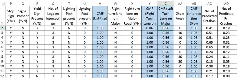
75 Table 4.16: 3ST Intersection Sample Worksheet 61

76 Table 4.17: Calculation of Calibration Factors for 3ST Intersections Method of Obtaining Observed Crashes at Intersections No. of Fatal Crashes No. of Injury Crashes Total (Fatal / Injury) Crashes No. of Property Damage Crashes Total (Fatal + Injury + Property Damage Only) No. of Daytime Crashes No. of Nighttime Crashes Nighttime Fatal Crash Nighttime Injury Crash Nighttime PDO Crash No. of Total Nighttime Crashes Predicted Total Crashes Predicted Fatal / Injury Crashes Intersection-Box (Method 1), Total Crash, C r = Fatal and Injury Crash, C r = Intersection-Related Crashes (Method 2), Total Crash, C r = Fatal and Injury Crash, C r = Total Observed Crashes = 53 = 2.87 Total Predicted Crashes Total Observed Crashes = 10 = 1.16 Total Predicted Crashes 8.59 Total Observed Crashes = 17 = 0.92 Total Predicted Crashes Total Observed Crashes = 4 = 0.47 Total Predicted Crashes 8.59 Using observed crashes within an intersection-box (method one), the obtained 0.91 calibration factor for total crashes on rural 4ST intersections indicated the closest crash prediction. The HSM underpredicts total crashes on 3ST intersections when considering crashes from method one but showed more accurate prediction when considering intersection-related crashes (method two). Fatal and injury crash prediction followed a similar trend for both methods of observed crashes. Results indicated that, using intersection-boxes (method one), the HSM is capable of predicting fatal and injury crashes when compared to actual observed crashes on rural 4ST and 3ST intersections. 62

77 Chapter 5: Development of Kansas-Specific New Safety Performance Functions for Rural Four-Lane Divided Segments The objective of this research was to calibrate the HSM for rural multilane highways, including segments and intersections, in Kansas. As discussed in Section 3.3, 4D and 4U segments were calibrated based on the HSM methodologies, and obtained calibration factors indicated that the HSM methodologies underpredict total crashes and overpredict fatal and injury crashes. In addition, the existing SPF given in the HSM was modified, resulting in satisfactory performance for total crash prediction. In order to obtain more reliable crash prediction, this study developed Kansas-specific SPFs and compared them to the HSM calibration and modified SPF method results. Developing jurisdiction-specific SPFs using data specific to each agency would potentially enhance reliability of the Part C predictive method. The HSM suggests that calibration of the jurisdiction-specific SPF using procedures in Appendix A of the HSM may not be necessary within the first 2 or 3 years after a jurisdiction-specific SPF is developed, especially if other default values in the HSM Part C models are replaced with locally derived values. 5.1 Model Selection for Kansas-Specific SPFs The first step in developing a new SPF is to determine which statistical method to use from the multiple statistical methods commonly used to create SPFs according to the literature review. Lord and Mannering (2010) identified promising models to be random-parameter models, finite mixture models, and Poisson and Negative Binomial regression models. The most popular current methods include Poisson regression, zero-inflated Poisson (ZIP) regression, and Negative Binomial regression models. The HSM (AASHTO, 2014) suggests using the Negative Binomial regression procedure because it accounts for overdispersion; however, many studies have successfully used Poisson regression during SPF development. Negative Binomial regression also accurately predicts crashes because it takes into account yearly crash variations and deviation from the normal variance. 63

78 Overdispersion occurs when the variance is larger than the sample mean. An overdispersion parameter indicates the statistical reliability of an SPF; a statistically reliable SPF should have an overdispersion parameter close to zero. A Negative Binomial regression model was considered in this study in order to obtain the best-performing model in compliance with the HSM. 5.2 Highway Segments for New SPF Development Among the 281 4D segments in this study, 200 randomly selected segments were considered for development of a new SPF; the remaining 81 segments were used for model validation. The random selection was performed using a random number generator in Microsoft Excel. All segments varied in length but maintained a minimum length of 0.1 miles. 5.3 New Variables Considered in Kansas-Specific SPFs SPFs in the HSM incorporate only segment length and AADT of 4D segments. However, the underprediction of total crashes indicated that other variables might be taken into account when predicting crashes for rural multilane segments in Kansas. After evaluating past studies and Kansas-specific attributes, several new variables were identified for consideration in the preliminary stage of SPF development. Differentiating between correlation and causality is difficult when selecting variables to model crashes. Correlation does not indicate the occurrence by the particular correlated factor. For example, correlation can occur between total crashes on a roadway segment and its length, even though the segment length did not cause the crashes. SPFs are simple because they often contain predictive rather than actual causal factors (Lord et al., 2008). Srinivasan and Carter (2011) found that segments within the influence of at-grade intersections and railroad grade crossings (250 ft on either side of at-grade intersections or railroad grade crossings) significantly affected crash prediction on rural segments. Therefore, all these factors were evaluated in this study during new SPF development. Speed limit, horizontal curve classification, gradient classification, presence of horizontal curve, presence of gradient, roadside hazard rating, medium truck volume, heavy truck volume, presence of rumble strips, and driveway density per mile 64

79 were potential variables considered in the Kansas-specific SPF development, as listed in Table 5.1. In addition to the independent variables given in the HSM, several new variables were considered in the Kansas-specific SPF development. Table 5.1: Variables in New SPF Development Variable Data Description Data Source L Segment Length AADT AADT LW Lane Width MW Median Width LSW Left Shoulder Width RSW Right Shoulder Width SS Side Slope SpL Speed Limit PHCur Presence of Horizontal Curve CANSYS Database C Curve Classifications G Presence of Gradient PG Gradient Classifications PRs Presence of Rumble Strips HTrc Heavy Truck Volume MTrc Medium Truck Volume TTrc Total Truck Volume RHR Roadside Hazard Rating DW Driveway Density per mile KDOT Videologs PL Presence of Lighting Google Maps Crashes Number of Crashes FI Crashes Number of Fatal and Injury Crashes KCARS Database Horizontal Alignment The CANSYS database provided horizontal curve classifications of roadway segments for this study. KDOT uses the same classification groups as the FHWA (shown in Table 5.2), and roadway segments have uniform alignment within the length. In developing the new SPF, 65

80 horizontal curve classification initially was a possible variable; for other model variations, however, presence of horizontal curve was considered to be a binomial variable (if present = 1, not present = 0). Table 5.2: Curve Classifications Curve Classification A B C D E F Degree of Curvature Under 3.5 degrees (i.e., radians) degrees (i.e., radians) degrees (i.e., radians) degrees (i.e., radians) degrees (i.e., radians) 28 degrees (i.e., radians) or more Vertical Grade The CANSYS database also provided vertical grades for this study. In developing the new SPF, vertical grade classification initially was a possible variable, but highways in rural Kansas do not contain much grade variation. Therefore, in the later models, presence of vertical grade was considered to be a binomial variable (if present = 1, not present = 0). Table 5.3 lists vertical grade classifications. Table 5.3: Vertical Grade Classifications Grade Classification Percent Grade A B C D E F 8.5 or greater 66

81 5.3.3 Roadside Hazard Rating The roadside hazard rating (RHR) is determined based on factors such as side slope, clear zone, and ability of a car to recover if it departed the roadway (Zegeer, Hummer, Reinfurt, Herf, & Hunter, 1987). Hazard ratings were assigned to each segment by comparing the side slope of the road from the CANSYS database to data from KDOT videologs and Google Street View. Because the topography of Kansas is fairly flat, the RHR for four-lane highways did not vary significantly along segments or among segments; RHR ranged from 1 to 4 (shown in Table 5.4), with 1 being the least hazardous and 4 being extremely hazardous. Table 5.4: Roadside Hazard Rating Criterion RHR Clear Zone Distance Side Slope Recoverable Special Features 1 >9 m (30 ft) from pavement edgeline Flatter than 1:4 Yes and 7.5 m (20 and 25 ft) from pavement edge line Approximately 1:4 Marginally Yes m (10 ft) from pavement edge line Approximately 1:3 to 1:4 Marginally Forgiving Rough roadside surface and 3 m (5 and 10 ft) from pavement edge line Approximately 1:3 or 1:4 Virtually No May have guardrail, exposed trees, poles, other objects Speed Limit Posted speed limit was another variable considered in the development of a new Kansasspecific SPF. Most segments had a posted speed limit of 65 mph, as taken from the CANSYS database. Segments had posted speed limits ranging from 50 to 70 mph Driveway Density Driveway density was determined using aerial photography in Google applications. Driveways onto the highway were counted and considered on a per-mile basis. Field entrances were disregarded because they are not used daily. Few segments had more than five driveways per mile, while many segments did not have any driveways. 67

82 Table 5.5 summarizes the mean, maximum, minimum, and standard deviation of data used in development of the new SPF for 4D segments. Table 5.5: Descriptive Statistics of Variables Description Average Min. Max. Std. Dev. Length (mile) AADT (vpd) 8, ,000 4,657 Left lane width (ft) Right lane width (ft) Left paved shoulder width (ft) Right paved shoulder width (ft) Median width (ft) Number of total crashes Number of fatal and injury crashes Presence of lighting Presence of rumble strips Posted speed limit (mph) Volume of medium truck (vpd) Volume of heavy truck (vpd) Total truck (vpd) , Gradient Presence of gradient Horizontal curve Presence of horizontal curve Roadside hazard rating No. of driveways per mile

83 5.4 Correlation Test Correlation analysis of variables was performed to identify correlation with total observed crashes and total fatal and injury crashes. Variables in the HSM include lane width, shoulder width, median width, total observed crashes, AADT, and length of segments. With the exception of segment length, none of the HSM variables showed strong correlation with total observed crashes at a 0.05 level of significance. Table 5.6 presents results of the correlation study, particularly the correlation of variables to total crashes and total fatal and injury crashes. A positive correlation indicates that as the variable increases, the amount of crashes also increases; a negative correlation indicates that as the variable increases, the number of crashes decreases. A significant correlation indicates a strong relationship between the data. Using a level of significance of 0.05, segment length, AADT, inner shoulder width, posted speed limit, presence of horizontal curve, and gradient class demonstrated statistically significant correlation in both crash categories. The presence of a rumble strip demonstrated significant correlation with total crashes only. Although correlation studies provide insight into the relationship between geometric features and crashes, they do not indicate cause and effect and can potentially be misleading. For example, according to Table 5.6, inner shoulder width has a positive correlation with both types of crashes, indicating that as inner shoulder width increases, the number of crashes increase. However, an increase in shoulder width typically is expected to decrease the number of crashes. Therefore, this relationship could have a confounding factor, thereby negatively affecting the correlation. 69

84 Table 5.6: Correlation Analysis of Variables Pearson s Correlation Coefficient (p-value) Variables Total Crashes Total Fatal and Injury Crashes Segment Length (mile) (<0.0001) (<0.0001) Median Width ( ) ( ) Inner Shoulder Width (0.0302) (0.0289) Outer Shoulder Width (0.0889) (0.1657) Lane Width (0.2737) (0.9728) Speed Limit (<.0001) (0.0001) AADT (<0.0001) (<0.0001) Volume of Medium Truck (0.276) (0.5313) Volume of Heavy Truck (0.0589) (0.3353) Total Truck (0.0691) (0.3443) Presence of Horizontal Curve (0.0241) (0.0476) Presence of Rumble Strip (0.0146) (0.244) Gradient Class (0.0467) (0.0474) Presence of Gradient (0.158) (0.1978) Presence of Lighting (0.0646) (0.3583) Driveways per Mile (0.0693) (0.128) Roadside Hazard Rating (0.8521) (0.8547) *highlighted variables indicate statistically significant correlation 70

85 5.5 New SPFs Once initial analysis of each variable was complete, the new SPFs were developed. Based on the HSM recommendations, Negative Binomial regression analysis was the model format, and new SPFs were created using Statistical Analysis Software (SAS) Total Crashes The first model for total crashes considered all geometric variables, AADT, segment length, classification of horizontal curve within segments, and classification of vertical gradient. The final model from this iteration was selected using the backward elimination process, including all statistically significant variables, as given in Equation 5.1 and Table 5.7. [ L AADT SpL] Prreeddiicctteedd CCrraassheess/yyeeaarr = ee Equation 5.1 Table 5.7: Parameter Estimates of Model 1 for Predicting Total Crashes Parameter DF Estimate Standard Error Chi- Square Pr > ChiSq Intercept Segment_Length < Speed_Limit AADT < Dispersion The second model considered the presence of horizontal curves and the presence of vertical gradients within segments instead of their classifications. The final model selected using the backward elimination process is given in Equation 5.2 and Table 5.8. Prreeddiicctteedd CCrraassheess/yyeeaarr = ee [ L AADT PHCrve SpL] Equation

86 Table 5.8: Parameter Estimates of Model 2 for Predicting Total Crashes Parameter DF Estimate Standard Error Chi- Square Pr > ChiSq Intercept < Segment_Length < Speed_Limit < AADT < Presence_of_Hor_Curve Dispersion The third model considered the natural logarithm of segment length, AADT, the presence of horizontal curves, and the presence of vertical gradients within segments. The final model selected using the backward elimination process is given in Equation 5.3 and Table 5.9. Prreeddiicctteedd CCrraassheess/yyeeaarr = ee [ Ln(L) Ln(AADT) PHCrve SpL MTrc ] Equation 5.3 Table 5.9: Parameter Estimates of Model 3 for Predicting Total Crashes Parameter DF Estimate Standard Error Chi- Square Pr > ChiSq Intercept < Ln_length < Speed_Limit Ln_AADT < Volume_of_Medium_Truck Presence_of_Hor_Curve Dispersion

87 The fourth model considered the natural logarithm of segment length, AADT, and total truck volume instead of heavy and medium truck volumes separately. The final model selected using the backward elimination process is given in Equation 5.4 and Table Prreeddiicctteedd CCrraassheess/yyeeaarr = ee [ Ln(L) Ln(AADT) PHCrve] Equation 5.4 Table 5.10: Parameter Estimates of Model 4 for Predicting Total Crashes Parameter DF Estimate Standard Error Chi- Square Pr > ChiSq Intercept < Ln_length < Ln_AADT < Presence_of_Hor_Curve Dispersion These models were compared using the stepwise selection process, which have similar significant variables with same model coefficients Fatal and Injury Crashes The first model for fatal and injury crashes considered all geometric variables, AADT, segment length, the classification of horizontal curves within segments, and the classification of vertical gradients. The first model from this iteration was selected using the backward elimination process, including all statistically significant variables, as given in Equation 5.5 and Table Prreeddiicctteedd CCrraassheess/yyeeaarr = ee [ L AADT LW RSW] Equation

88 Table 5.11: Parameter Estimates of Model 1 for Predicting Fatal and Injury Crashes Parameter DF Estimate Standard Error Chi- Square Pr > ChiSq Intercept Segment_Length < Right_Shoulder_Width AADT < Lane_Width Dispersion The second model considered the presence of horizontal curves and vertical gradients within segments instead of their classifications. The final model selected using the backward elimination process is given in Equation 5.6 and Table [ L AADT LW + Prreeddiicctteedd CCrraassheess/yyeeaarr = ee SpL] Equation 5.6 Table 5.12: Parameter Estimates of Model 2 for Predicting Fatal and Injury Crashes Parameter DF Estimate Standard Error Chi- Square Pr > ChiSq Intercept Segment_Length < Speed_Limit AADT < Lane_Width Dispersion

89 The third model considered the natural logarithm of segment length, AADT, the presence of horizontal curves, and the presence of vertical gradients within segments. The final model selected using the backward elimination process is given in Equation 5.7 and Table [ Ln(L) Ln(AADT) LW MTrc] Prreeddiicctteedd CCrraassheess/yyeeaarr = ee Equation 5.7 Table 5.13: Parameter Estimates of Model 3 for Predicting Fatal and Injury Crashes Parameter DF Estimate Standard Error Chi- Square Pr > ChiSq Intercept < Ln_length < Volume_of_Med_Truck Lane_Width Ln_AADT < Dispersion The fourth model considered the natural logarithm of segment length, AADT, and total truck volume instead of heavy and medium truck volumes separately. The final model selected using the backward elimination process is given in Equation 5.8 and Table [ Lnn(L) Lnn(AADT) LW ] Prreeddiicctteedd CCrraassheess/yyeeaarr = ee Equation 5.8 Where: L = segment length, LW = lane width, SpL = speed limit, HTrc = volume of heavy truck, MTrc = volume of medium truck, DW = driveways per mile, RSW = right shoulder width, and PHCur = presence of horizontal curve. 75

90 Table 5.14: Parameter Estimates of Model 4 for Predicting Fatal and Injury Crashes Parameter DF Estimate Standard Error Chi- Square Pr > ChiSq Intercept < Ln_length < Lane_Width Ln_AADT < Dispersion Validation Once the SPFs were developed, they were validated using a set of roadway segments that differed from the segments used to create new SPFs. Statistical tests were run to determine which model was better and could be observed if results match with known guidelines. Bayesian information criterion (BIC), Akaike information criterion (AIC), and corrected Akaike information criterion (AICc) are some of the methods and tests that were performed to obtain best models Total Crashes Table 5.15 compares the goodness of fit for all models developed to predict total crashes, summarizing goodness-of-fit indicators such as log-likelihood, AIC, AICc, and BIC. As shown in the table, Model 4 demonstrated an overall better fit than Models 1, 2, or 3. The criterion on loglikelihood was not clearly mentioned in most cases, and it alone cannot be used to assess a model. However, a previous study proved that a high log-likelihood is an indication of a better model (Caliendo, Guida, & Parisi, 2007). AIC, AICc, and BIC indicated smaller values to be representative of better fit; results indicated that consideration of the natural logarithm of segment length and AADT (Equation 5.4) more accurately explains total crashes on rural multilane highways in Kansas. 76

91 Table 5.15: Goodness-of-Fit Comparison for Total Crashes Model Criterion Model 1 Model 2 Model 3 Model 4 Model Goodnessof-Fit Criteria Deviance/df Scaled Deviance/df Pearson Chi- Square/df Scaled Pearson Chi-Square/df Log-Likelihood Higher is better Full Log-Likelihood Higher is better AIC Smaller is better AICc Smaller is better BIC Smaller is better Each model was run through the validation dataset that consisted of segments not used during development of the new SPF. The number of predicted crashes at each segment, as obtained though the validation process, were plotted against observed crashes. Figures 5.1, 5.2, 5.3, and 5.4 show plots of predicted crashes compared to observed crashes for Models 1, 2, 3, and 4, respectively, in order to identify the best model for crash prediction. Ideally, the predicted crashes should be equal or approximately close to the actual observed crashes. The trend line of each plot indicates the plot fit. If predicted crashes and observed crashes are identical, then R 2 is Among the four graphs, Model 4 demonstrated closest predicted crashes compared to other models; therefore, this model is the best option to predict total crashes on rural four-lane highways in Kansas. 77

92 Predicted Crashes y = x R² = Observed Crashes Figure 5.1: Total Crashes: Model 1 Validation Plot Predicted Crashes y = x R² = Observed Crashes Figure 5.2: Total Crashes: Model 2 Validation Plot 78

93 Predicted Crashes y = x R² = Observed Crashes Figure 5.3: Total Crashes: Model 3 Validation Plot y = x R² = Predicted Crashes Observed Crashes Figure 5.4: Total Crashes: Model 4 Validation Plot Outlier Analysis In order to obtain the best-fitted model, analysis was performed to identify possible outliers or influential data points. Studentized residuals and studentized deleted residuals were used to identify such locations. 79

94 Studentized Residual An outlier is a point with a response variable that is far from the implied general regression relationship, thereby requiring a large residual (in absolute value). Studentized residuals (or internally studentized residuals) are defined for each observation, i = 1, 2..., n, as an ordinary residual divided by an estimate of its standard deviation. z i * = y i y i MSE 1 h i Equation 5.9 Where: yy ii = Observation i, yy ii = Predicted response if observation i is removed from model, MSE = Mean standard error, and h i = Leverage. Leverage measures the influence of the observation. Any observation with a studentized residual larger than 3 (in absolute value) is generally deemed an outlier. Studentized Deleted Residual Studentized deleted residual is residual divided by the standard deviation of the residual, or a residual standardized to have a standard deviation of 1. More precisely, the i th standardized residual equals: d i * = y i y i stanndard error d i * > t Equation 5.10 df = (n -1) (k +1) Equation 5.11 Where: n = Sample size, and k = Number of predictors. Using outputs of each model, residuals were generated via SAS. Validation segments that showed studentized residual greater than 3 were considered outliers. Segments that showed studentized deleted residual greater than t were also identified as outliers. Figures 5.5, 5.6, 5.7, and 5.8 show plots of predicted total crashes compared to observed crashes after outliers 80

95 were removed. These figures indicate that removal of outliers improved model fit since R 2 of each plot increased. However, even after outliers were removed, Model 4 was still the best model. 350 Number of Predicted Crashes y = x R² = Observed Crashes Figure 5.5: Total Crashes: Model 1 Validation Plot (Without Outliers) 350 Number of Predicted Crashes y = x R² = Observed Crashes Figure 5.6: Total Crashes: Model 2 Validation Plot (Without Outliers) 81

96 80 Number of Predicted Crashes y = x R² = Observed Crashes Figure 5.7: Total Crashes: Model 3 Validation Plot (Without Outliers) Number of Predicted Crashes y = 0.685x R² = Observed Crashes Figure 5.8: Total Crashes: Model 4 Validation Plot (Without Outliers) Fatal and Injury Crashes Table 5.16 compares goodness of fit for all models developed to predict fatal and injury crashes, summarizing goodness-of-fit indicators such as log-likelihood, AIC, AICc, and BIC. As shown in the table, Model 4 had an overall better fit than Models 1, 2, and 3 because it had a 82

97 goodness of fit between 0.8 and 1.2. Although log-likelihood criterion is not clearly mentioned in most cases and it alone cannot be used to assess a model, a previous study (Caliendo et al., 2007) proved that a high log-likelihood indicates a better model. AIC, AICc, and BIC indicate smaller values to be the representative of better fit. Results indicated that consideration of the natural logarithm of segment length and AADT more accurately explains fatal and injury crashes on rural multilane highways in Kansas. Table 5.16: Goodness-of-Fit Comparison of Fatal and Injury Crash Models Criterion Model 1 Model 2 Model 3 Model 4 Model Goodnessof-Fit Criteria Deviance/df Scaled Deviance/df Pearson Chi- Square/df Scaled Pearson Chi- Square/df Log-Likelihood Higher is better Full Log-Likelihood Higher is better AIC Smaller is better AICc Smaller is better BIC Smaller is better Each model was run through the validation dataset that consisted of segments not used during the development of the new SPF. The number of predicted crashes at each segment, as obtained though the validation process, were plotted against observed crashes. Figures 5.9, 5.10, 5.11, and 5.12 show plots of predicted fatal and injury crashes compared to observed crashes corresponding to Models 1, 2, 3, and 4, respectively. Results from Model 4 demonstrated closest predicted crashes, so this model is the best option to predict fatal and injury crashes on rural four-lane highways in Kansas. 83

98 25 Predicted Crashes y = x R² = Observed Crashes Figure 5.9: Fatal and Injury Crashes: Model 1 Validation Plot Predicted Crashes y = x R² = Observed Crashes Figure 5.10: Fatal and Injury Crashes: Model 2 Validation Plot 84

99 14 Predicted Crashes y = x R² = Observed Crashes Figure 5.11: Fatal and Injury Crashes: Model 3 Validation Plot 12 Predicted Crashes y = x R² = Observed Crashes Figure 5.12: Fatal and Injury Crashes: Model 4 Validation Plot Outlier Analysis Residuals were generated via SAS using model outputs. Validation segments showing studentized residual greater than 3 were considered outliers. Segments showing studentized deleted residual greater than t 0.00 were also identified as outliers. Figures 5.13, 5.14, 5.15, and 5.16 show plots of predicted total crashes compared to observed crashes after outliers were 85

100 removed. As shown in the figures, removing the outliers improved model fit since R 2 of each plot increased. However, even after outliers were removed, Model 4 was still the best model. Predicted Crashes y = x R² = Observed Crashes Figure 5.13: Fatal and Injury Crashes: Model 1 Validation Plot (Without Outliers) Predicted Crashes y = x R² = Observed Crashes Figure 5.14: Fatal and Injury Crashes: Model 2 Validation Plot (Without Outliers) 86

101 14 Predicted Crashes y = x R² = Observed Crashes Figure 5.15: Fatal and Injury Crashes: Model 3 Validation Plot (Without Outliers) Predicted Crashes y = x R² = Observed Crashes Figure 5.16: Fatal and Injury Crashes: Model 4 Validation Plot (Without Outliers) 5.7 Comparison of New SPF to HSM-given SPF The new Kansas-specific SPFs were compared to the HSM calibration and modified HSM-given SPF for predicted crashes. Errors in prediction compared to observed data were obtained to calculate Mean Prediction Bias (MPB), Mean Absolute Deviation (MAD), and Mean Squared Predicted Error (MSPE). Table 5.17 compares model statistics in which statistical parameters close to 0 indicate a desirable model and good fit of the data (Garber et al., 2011). Since positive MPB indicates overprediction and negative MPB indicates underprediction, the new SPF showed the least 87

102 underprediction for total crashes, and the modified HSM model showed the least underprediction for fatal and injury crashes. The new SPF showed smallest MAD, indicating the best fit for predicting total crashes and fatal and injury crashes. Similarly, smaller MSPE indicates a better fit, and the Kansas-specific SPF showed optimal results. Therefore, the new Kansas-specific SPF for four-lane divided highway segments more accurately predicts total and fatal and injury crashes for rural Kansas. Table 5.17: Comparison of Model Statistics Model MPB MAD MSPE HSM Total Crashes Modified HSM Total Crashes New SPF Total Crashes HSM Fatal and Injury Crashes Modified HSM Fatal and Injury Crashes New SPF Fatal and Injury Crashes

103 Chapter 6: Summary, Conclusions, and Recommendations 6.1 Summary and Conclusions The HSM is commonly used to predict crash frequency for highway facilities using SPFs that were developed based on available crash and other data throughout several states. The HSM recommends that models be calibrated based on crash data from the local jurisdiction in order to obtain a more reliable crash prediction. An acceptable method to predict crashes for rural multilane highway segments and intersections in Kansas must be developed if calibration does not lead to accurate predictions. Prior to this study, the Kansas Department of Transportation (KDOT) could apply the rural two-lane model given in the HSM, but rural multilane highways in Kansas were lacking a reliable crash prediction methodology. KDOT has occasionally requested analysis of a multilane facility, but it could not be completed without calibration. The objective of this research was to calibrate the HSM for rural multilane highways in Kansas that include 4D and 4U segments and 4ST and 3ST intersections. As discussed in Section 3.3, 4D and 4U segments were calibrated based on the HSM methodologies. Obtained calibration factors indicated that the HSM methodologies underpredict total crashes and overpredict fatal and injury crashes. The corresponding calibration factors can be used for future crash prediction. Several default regression factors and crash proportions are utilized in the HSM calibration methodology. A comparison of Kansas crash proportions based on severity, daytime/nighttime condition, and collision type revealed significant differences between these proportions and default crash proportions in the HSM. The HSM-given SPF regression coefficients were therefore modified to capture variations in crash predictions to better suit Kansas conditions. The SPFs with new coefficients were multiplied by CMFs to obtain the predicted crash frequency. The adjusted models for 4D and 4U facilities indicated significant improvement in crash prediction compared to HSM crash prediction for rural Kansas. Kansas-specific SPFs were developed in this study according to the HSM recommendations (AASHTO, 2014). Development of jurisdiction-specific SPFs using individual agency data typically enhanced reliability of Part C predictive methods in the HSM. The HSM suggests, however, that calibration of jurisdiction-specific SPFs using procedures in the Appendix A of the HSM may not be necessary within the first 2 or 3 years after development, 89

104 particularly if other default values in the HSM Part C models are replaced with locally derived values. Analysis results showed two models that would work best for the state of Kansas. One model predicts total crashes better, and the other model predicts fatal and injury crashes better. The model for predicting total crashes includes segment length, AADT, and the presence of horizontal curves. The model for predicting fatal and injury crashes in Kansas included segment length, AADT, and lane width as significant variables. This model showed smallest BIC, AIC, and AICc and high log-likelihood in the goodness-of-fit tests. The newly developed SPFs were also compared to the HSM-given SPF and adjusted SPF using the statistical parameters Mean Prediction Bias, Mean Absolute Deviation, and Mean Squared Prediction Error, leading to the conclusion that the new Kansas-specific SPF for 4D highway segments reliably predicts total and fatal and injury crashes in rural Kansas. This model fits Kansas data better than the HSM-given SPF and modified SPF, thereby enabling prediction closest to actual conditions. However, if geometric data are not readily available, then the modified SPF would be a better alternative because it has fewer data requirements than the other models. In addition to segments, this study calibrated multilane intersections. The HSM methodology was followed to obtain the number of predicted crashes at 4ST and 3ST intersections. Observed crashes at intersections were considered using two methods: intersectionboxes and intersection-related crashes. This study found that intersection-box crashes (method one) predict the fatal and injury crashes comparatively close to actual observed crashes on rural 4ST and 3ST intersections. The number of predicted crashes at segments and intersections can be used for several situations such as: comparing facilities under past or future traffic volumes, checking the alternative designs for an existing facility, designing a new facility under future traffic volumes, estimating effectiveness of countermeasures after a period of implementation, and estimating effectiveness of a proposed countermeasure on an existing facility prior to implementation. This research will help private, county, and state agencies identify possible factors that may influence rural crash occurrence and help determine if a countermeasure could reduce rural 90

105 fatalities. Calibration of the HSM predictive model for multilane facilities will help transportation practitioners reduce the number of fatalities on rural roadways in Kansas. Development of reliable crash prediction methodology will ultimately save lives in Kansas and reduce the number of crashes and fatalities on rural multilane roadways and intersections. 6.2 Recommendations and Future Work Additional work could further improve the reliability of Kansas-specific crash prediction models, including considering additional CMFs and determining their effect on crash prediction. The HSM suggests that local CMFs be developed if agencies believe that factor has a significant effect on crash frequencies. Because Kansas highways are not geographically similar in all districts or even counties and terrain differences exist throughout the state, development of county-specific and zone-specific (north, south, east, and west) calibration factors for rural multilane segments and intersections may be checked to verify whether separate calibration increases the reliability of crash prediction. The literature review included studies that have considered separate analysis for multiple zones within a single state. Sample size was the biggest challenge while analyzing rural multilane intersections. In future work, sample size should be increased to increase the degrees of freedom and allow consideration of various regression types in order to increase the likelihood of statistically significant explanatory variables. The database of highway intersections should also continue to be expanded until it includes all geometric features of the Kansas highway system. In addition, methodologies described in this report would provide closer crash prediction with a larger sample size. 91

106 References Alluri, P., & Ogle, J. (2012). Effects of state-specific SPFs, AADT estimations, and overdispersion parameters on crash predictions using SafetyAnalyst (Paper No ). In TRB 91st Annual Meeting compendium of papers. Washington, DC: Transportation Research Board. Alluri, P., Saha, D., Liu, K., & Gan, A. (2014). Improved Processes for meeting the data requirements for implementing the Highway Safety Manual (HSM) and SafetyAnalyst in Florida. Tallahassee, FL: Florida Department of Transportation. American Association of State Highway and Transportation Officials (AASHTO). (2014). Highway safety manual, first edition, with 2014 supplement. Washington, DC: Author. Banihashemi, M. (2011). Highway Safety Manual, new model parameters vs. calibration of crash prediction models (Paper No ). In TRB 90th Annual Meeting compendium of papers. Washington, DC: Transportation Research Board. Banihashemi, M. (2012). Sensitivity analysis of data set sizes for Highway Safety Manual calibration factors. Transportation Research Record, 2279, Bornheimer, C. (2011). Finding a new safety performance function for two-way, two-lane highways in rural areas (Master s thesis). University of Kansas, Lawrence, KS. Bornheimer, C., Schrock, S.D., Wang, M.H., & Lubliner, H. (2012). Developing a regional safety performance function for rural two-lane highways (Paper No ). In TRB 91st Annual Meeting compendium of papers. Washington, DC: Transportation Research Board. Caliendo, C., Guida, M., & Parisi, A. (2007). A crash-prediction model for multilane roads. Accident Analysis & Prevention, 39(4), Dixon, K., Monsere, C., Xie, F., & Gladhill, K. (2012). Calibrating the future Highway Safety Manual predictive methods for Oregon state highways (Report No. FHWA-OR-RD-12-07). Salem, OR: Oregon Department of Transportation. Garber, N.J., Rivera, G., & Lim, I.K. (2011). Safety performance functions for intersections in Virginia (Paper No ). In TRB 90th Annual Meeting compendium of papers. Washington, DC: Transportation Research Board. 92

107 Garber, N.J., & Wu, L. (2001). Stochastic models relating crash probabilities with geometric and corresponding traffic characteristics data (Report No. UVACTS ). Charlottesville, VA: Center for Transportation Studies, University of Virginia. Google. (n.d.). Google Maps. Retrieved from Heron, M. (2016). Deaths: Leading causes for National Vital Statistics Reports, 65(2), Retrieved from Hilbe, J.M. (2011). Negative binomial regression. Cambridge, UK: Cambridge University Press. Jalayer, M., Zhou, H., Williamson, M., & LaMondia, J.J. (2015). Developing calibration factors for crash prediction models with consideration of crash recording threshold change (Paper No ). In TRB 94th Annual Meeting compendium of papers. Washington, DC: Transportation Research Board. Kansas Department of Transportation (KDOT). (2005). Kansas motor vehicle accident report coding manual. Topeka, KS: Author. Kansas Department of Transportation (KDOT). (2011). Data support: The data team. Retrieved April 12, 2015, from Kansas Department of Transportation (KDOT). (2012) Kansas traffic accident facts: Definitions. Retrieved April 12, 2015, from k/definitions.pdf Kansas Department of Transportation (KDOT). (2015a). Kansas transportation quick facts. Retrieved March 14, 2016, from Kansas Department of Transportation (KDOT). (2015b). Kansas mileage and travel by functional classification Retrieved March 14, 2016, from vel/funclass2014.pdf 93

108 Kweon, Y.J., Lim, I.K., Turpin, T.L., & Read, S.W. (2014). Development and application of guidance to determine the best way to customize the Highway Safety Manual for Virginia (Paper No ). In TRB 93rd Annual Meeting compendium of papers. Washington, DC: Transportation Research Board. Long, J.S. (1997). Regression models for categorical and limited dependent variables. Thousand Oaks, CA: SAGE Publications, Inc. Lord, D., Geedipally, S.R., Persaud, B.N., Washington, S.P., van Schalkwyk, I., Ivan, J.N., Jonsson, T. (2008). Methodology to predict the safety performance of rural multilane highways (NCHRP Web-Only Document 126). Washington, DC: Transportation Research Board. Lord, D., & Mannering, F. (2010). The statistical analysis of crash-frequency data: A review and assessment of methodological alternatives. Transportation Research Part A: Policy and Practice, 44(5), Lubliner, H. (2011). Evaluation of the Highway Safety Manual crash prediction model for rural two-lane highway segments in Kansas (Doctoral dissertation). University of Kansas, Lawrence, KS. Lubliner, H., & Schrock, S.D. (2012). Calibration of the Highway Safety Manual prediction method for rural Kansas highways (Paper No ). In TRB 91st Annual Meeting compendium of papers. Washington, DC: Transportation Research Board. Mehta, G., & Lou, Y. (2013). Calibration and development of safety performance functions for Alabama: Two-lane, two-way rural roads and four-lane divided highways. Transportation Research Record, 2398, Miaou, S.P., & Lum, H. (1993). Statistical evaluation of the effects of highway geometric design on truck accident involvements. Transportation Research Record, 1407, Najjar, Y., & Mandavilli, S. (2009). Data mining the Kansas Traffic-Crash Database (Report No. K-TRAN: KSU-05-6). Topeka, KS: Kansas Department of Transportation. National Highway Traffic Safety Administration (NHTSA). (2009). Traffic safety facts Retrieved April 4, 2015, from 94

109 National Highway Traffic Safety Administration (NHTSA). (2016). Quick facts Retrieved March 14, 2016, from Qin, X., Zhi, C., & Vachal, K. (2014). Calibration of Highway Safety Manual predictive methods for rural local roads (Paper No ). In TRB 93rd Annual Meeting compendium of papers. Washington, DC: Transportation Research Board. Shin, H., Lee, Y.J., & Dadvar, S. (2014). The development of local calibration factors for implementing the Highway Safety Manual in Maryland (Report No. MD-14-SP209B4J). Hanover, MD: Maryland State Highway Administration. Srinivasan, R., & Carter, D. (2011). Development of safety performance functions for North Carolina (Report No. FHWA/NC/ ). Raleigh, NC: North Carolina Department of Transportation. Sun, C., Edara, P., Brown, H., Claros, B., & Nam, K. (2013). Calibration of the Highway Safety Manual for Missouri (Report No. cmr14-007). Jefferson City, MO: Missouri Department of Transportation. Sun, X., Li, Y., Magri, D., & Shirazi, H.H. (2006). Application of Highway Safety Manual draft chapter: Louisiana experience. Transportation Research Record, 1950, Sun, X., Magri, D., Shirazi, H.H., Gillella, S., & Li, L. (2011). Application of Highway Safety Manual: Louisiana experience with rural multilane highways (Paper No ). In TRB 90th Annual Meeting compendium of papers. Washington, DC: Transportation Research Board. Xie, F., Gladhill, K., Dixon, K.K., & Monsere, C.M. (2011). Calibration of Highway Safety Manual predictive models for Oregon state highways. Transportation Research Record, 2241, Zegeer, C.V., Hummer, J., Reinfurt, D., Herf, L., & Hunter, W. (1987). Safety effects of crosssection design for two-lane roads: Volume I (Report No. FHWA-RD-87/008). McLean, VA: Federal Highway Administration. 95

110 Appendix: Calibration Data Table A.1: List of Locations for 4D Segment Calibration ID Route Id Prefix Route Dir Begin County Milepost End County Milepost Segment Length (mile) AADT U EB U EB U NB U NB U NB U NB U NB U NB U NB U NB U NB U NB U NB U NB U NB U NB U NB U NB K EB K EB K EB K EB K EB K EB K EB K EB K EB K EB K EB K EB U EB U EB U EB U EB U EB U EB U EB U EB U EB U EB U EB U EB U EB U EB U EB U EB U NB U NB U NB U NB K EB K EB K EB K EB K EB K EB K EB K EB K EB K EB U NB U NB U NB U NB U SB U SB U SB U SB U SB U SB U SB U SB U SB U SB U SB U SB U SB U SB U SB U SB U SB U SB U SB U SB

111 ID Route Id Prefix Route Dir Begin County Milepost End County Milepost Segment Length (mile) AADT U NB U NB U NB U NB U NB U NB U NB U NB U NB U NB U NB U NB U NB U NB U NB U NB U NB U NB U NB U NB U NB U NB U NB U NB U NB U NB U NB U NB K EB K EB K EB K EB K EB K EB U NB U NB U NB U NB U NB U NB U EB U EB U EB U EB U EB U EB U EB U EB U EB U EB U EB U EB U EB U EB U NB U NB U NB U NB U NB U NB U NB U NB U NB U NB K EB K EB K EB K EB K EB K EB K NB K NB K NB K NB U EB U EB U EB U EB U NB U NB U NB U NB U NB U NB U NB U NB U NB U NB U EB U EB

112 ID Route Id Prefix Route Dir Begin County Milepost End County Milepost Segment Length (mile) AADT U EB U EB U EB U EB U EB U EB U EB U EB K EB K EB K EB K EB K EB K EB K EB K EB U NB U NB U NB U NB U NB U NB U NB U NB U EB U EB U EB U EB U EB U EB U EB U EB U EB U EB U EB U EB U EB U EB U EB U EB U EB U EB U EB U EB U EB U EB U EB U EB U EB U EB U EB U EB U EB U EB U EB U EB U EB U EB U EB U EB U EB U EB U EB U EB U EB U EB U EB U EB U EB U EB U EB U EB U EB U EB U EB U EB U EB U EB U SB U SB U SB U SB U SB U SB U SB U SB U SB U SB U SB U SB

113 ID Route Id Prefix Route Dir Begin County Milepost End County Milepost Segment Length (mile) AADT U SB U SB U SB U SB U SB U SB U EB U EB U EB U EB U EB U EB U EB U EB K NB K NB K NB K NB K NB K NB K NB K NB K NB K NB K NB K NB K NB K NB K NB K NB K NB K NB K NB K NB K NB K NB U00081B1-NB U NB U EB U EB U EB U EB U NB U NB U NB U NB U NB U NB U NB U NB U NB U NB U NB U NB U NB U NB U NB U NB U NB U NB U NB U NB U NB U NB U NB U NB U NB U NB U NB U NB U WB U WB U WB U WB U EB U EB U EB U EB U EB U EB U NB U NB U NB U NB U NB U NB U NB U NB U NB U NB

114 ID Route Id Prefix Route Dir Begin County Milepost End County Milepost Segment Length (mile) AADT U NB U NB U NB U NB U NB U NB U SB U SB U SB U SB U SB U SB U EB U EB K NB K NB U NB U NB U NB U NB U NB U NB U NB U NB U NB U NB U NB U NB U NB U NB U NB U NB U NB U NB U SB U SB U SB U SB U SB U SB U SB U SB U SB U SB U SB U SB U SB U SB U WB U WB U WB U WB U WB U WB K NB K NB U EB U EB U EB U EB K WB K WB K WB K WB K WB K WB K WB K WB K NB K NB K NB K NB K NB K NB K NB K NB K EB K EB K EB K EB K EB K EB K EB K EB K EB K EB U WB U WB U WB U WB

115 ID Route Id Prefix Route Dir Begin County Milepost End County Milepost Segment Length (mile) AADT U WB U WB U WB U WB U WB U WB U NB U NB U NB U NB U NB U NB U NB U NB U NB U NB U NB U NB U NB U NB U NB U NB U NB U NB U NB U NB U NB U NB U NB U NB U NB U NB U NB U NB U SB U SB U SB U SB U SB U SB U SB U SB U SB U SB U SB U SB U SB U SB U SB U SB U SB U SB K EB K EB K NB K NB K EB K EB U NB U NB K EB K EB U NB U NB U NB U NB K EB K EB K EB K EB K EB K EB K EB K EB K EB K EB K EB K EB K EB K EB U EB U EB U EB U EB U EB U EB U EB U EB U EB U EB

116 ID Route Id Prefix Route Dir Begin County Milepost End County Milepost Segment Length (mile) AADT U EB U EB U EB U EB U EB U EB U EB U EB U EB U EB U EB U EB U EB U EB U NB U NB U SB U SB U SB U SB U EB U EB U EB U EB U NB U NB U EB U EB

117 Table A.2: List of Locations for 4U Segment Calibration ID Route Id Prefix Route Dir Begin County Milepost End County Milepost Segment Length (mile) AADT U EB U EB U EB U EB U EB U EB U EB U EB U EB U EB U EB U EB U EB U EB U EB U EB U EB U EB U NB U NB U EB U EB U EB U EB U NB U NB U NB U NB U EB U EB U EB U EB U EB U EB U EB U EB U EB U EB U EB U EB U EB U EB K EB K EB U NB U NB K EB K EB U EB U EB U EB U EB U EB U EB U EB U EB U EB U EB U EB U EB U EB U EB U EB U EB U EB U EB U EB U EB U EB U EB U EB U EB U EB U EB U NB U NB U NB U NB U EB U EB U EB U EB U EB U EB U EB U EB U EB U EB

118 ID Route Id Prefix Route Dir Begin County Milepost End County Milepost Segment Length (mile) AADT U EB U EB U EB U EB U EB U EB U EB U EB K EB K EB U NB U NB U NB U NB U NB U NB U NB U NB U NB U NB U EB U EB U EB U EB U EB U EB K EB K EB U NB U NB U EB U EB U EB U EB U EB U EB U NB U NB K NB K NB U EB U EB U EB U EB U EB U EB U EB U EB U EB U EB U EB U EB U EB U EB U EB U EB U EB U EB U EB U EB U EB U EB U EB U EB U EB U EB U EB U EB U EB U EB U EB U EB U EB U EB U EB U EB U EB U EB

119 Intersection ID Section ID Table A.3: List of Locations for 4ST Intersections Calibration County Name Highway No. Begin County MP End County MP Direction (EB/WB/NB/SB) Number of all crashes within ints. box of 300 ft Number of intersection related crashes (only) 1 67 FINNEY US EB FINNEY US EB FINNEY US EB LEAVENWORTH US EB PRATT K EB REPUBLIC US NB SEDGWICK US EB ALLEN US EB BOURBON US NB BOURBON US NB BOURBON US NB BUTLER K EB BUTLER K EB BUTLER K EB BUTLER K EB BUTLER K EB BUTLER K EB BUTLER K EB BUTLER K EB BUTLER K EB BUTLER K EB BUTLER K EB BUTLER US EB BUTLER US EB BUTLER US EB BUTLER US EB BUTLER US EB BUTLER US EB BUTLER US EB BUTLER US EB BUTLER US EB BUTLER US EB BUTLER US EB BUTLER US EB BUTLER US EB BUTLER US EB BUTLER US NB BUTLER US NB CHEROKEE K EB CHEROKEE K EB CHEROKEE K EB CLOUD US NB CLOUD US NB

120 Intersection ID Section ID County Name Highway No. Begin County MP End County MP Direction (EB/WB/NB/SB) Number of all crashes within ints. box of 300 ft Number of intersection related crashes (only) CLOUD US NB CLOUD US NB CLOUD US SB CLOUD US SB CLOUD US SB CLOUD US SB CLOUD US SB CLOUD US SB CLOUD US SB CLOUD US SB CLOUD US SB CLOUD US SB CLOUD US SB CLOUD US SB COWLEY US NB COWLEY US NB COWLEY US NB COWLEY US NB COWLEY US NB COWLEY US NB COWLEY US NB COWLEY US NB COWLEY US NB COWLEY US NB CRAWFORD US NB JACKSON US NB JACKSON US NB JACKSON US NB JACKSON US EB JACKSON US EB JACKSON US EB JACKSON US EB MARSHALL US EB MARSHALL US EB MARSHALL US EB POTTAWATOMIE US WB POTTAWATOMIE US WB POTTAWATOMIE US WB POTTAWATOMIE US WB POTTAWATOMIE US WB POTTAWATOMIE US WB POTTAWATOMIE US WB POTTAWATOMIE US WB POTTAWATOMIE US WB

121 Intersection ID Section ID County Name Highway No. Begin County MP End County MP Direction (EB/WB/NB/SB) Number of all crashes within ints. box of 300 ft Number of intersection related crashes (only) POTTAWATOMIE US WB POTTAWATOMIE US WB POTTAWATOMIE US WB POTTAWATOMIE US WB POTTAWATOMIE US WB PRATT K NB RENO K WB RENO K WB RENO K WB RENO K EB RENO K EB RENO K EB RENO K EB RENO K EB RENO K EB RENO K EB RENO K EB RENO K EB RENO K EB RENO US WB RENO US WB RENO US WB REPUBLIC US NB REPUBLIC US NB REPUBLIC US NB REPUBLIC US NB REPUBLIC US NB REPUBLIC US NB REPUBLIC US NB REPUBLIC US NB REPUBLIC US NB REPUBLIC US NB REPUBLIC US NB REPUBLIC US NB REPUBLIC US NB REPUBLIC US NB REPUBLIC US NB REPUBLIC US NB REPUBLIC US SB REPUBLIC US SB REPUBLIC US SB REPUBLIC US SB REPUBLIC US SB REPUBLIC US SB

122 Intersection ID Section ID County Name Highway No. Begin County MP End County MP Direction (EB/WB/NB/SB) Number of all crashes within ints. box of 300 ft Number of intersection related crashes (only) REPUBLIC US SB REPUBLIC US SB REPUBLIC US SB REPUBLIC US SB REPUBLIC US SB ROOKS K EB RUSSELL US NB SEDGWICK K EB SEDGWICK K EB SEDGWICK K EB SEDGWICK K EB SEDGWICK K EB SEDGWICK K EB SEDGWICK K EB SEDGWICK K EB SEDGWICK K EB SEDGWICK K EB SEDGWICK K EB SEDGWICK K EB SEDGWICK US EB SEWARD US EB SHAWNEE US SB SHAWNEE US SB SHAWNEE US SB SHAWNEE US SB SHAWNEE US SB SHAWNEE US SB WASHINGTON US EB WASHINGTON US EB WASHINGTON US EB WASHINGTON US EB WASHINGTON US EB WILSON US NB WILSON US NB WILSON US NB ALLEN US EB ALLEN US EB ALLEN US EB ALLEN US EB ANDERSON US NB BARTON US EB BARTON US NB BROWN US NB BROWN US NB

123 Intersection ID Section ID County Name Highway No. Begin County MP End County MP Direction (EB/WB/NB/SB) Number of all crashes within ints. box of 300 ft Number of intersection related crashes (only) CHEROKEE US EB CHEROKEE US EB CHEROKEE US EB CHEYENNE US EB FINNEY US EB GEARY K EB GRAHAM US EB HASKELL US EB JACKSON US NB LYON US EB OSAGE US EB OSAGE US EB OSBORNE US EB OSBORNE US EB OSBORNE US EB POTTAWATOMIE US EB POTTAWATOMIE US EB REPUBLIC US EB ROOKS US EB STAFFORD US NB STEVENS US EB THOMAS US EB WALLACE US EB WALLACE US EB

124 Intersection ID Section ID Table A.4: List of Locations for 3ST Intersections Calibration County Name Highway No. Begin County MP End County MP Direction (EB/WB/NB/SB) Number of all crashes within ints. box of 300 ft Number of intersection related crashes (only) 1 2 ALLEN US EB ALLEN US EB ALLEN US EB ALLEN US EB ALLEN US EB ALLEN US EB ALLEN US EB BARTON US NB BARTON US NB BARTON US NB BOURBON US NB BUTLER US NB CHEROKEE US EB DECATUR US NB GOVE US EB GRAHAM US EB GRAHAM US EB GRAHAM US EB GRAHAM US EB GRAHAM US EB JEWELL US EB MARION K NB MARSHALL US EB MONTGOMERY US NB MONTGOMERY US NB NEMAHA US EB NEMAHA US EB NEMAHA US EB OSBORNE US EB OSBORNE US EB POTTAWATOMIE US EB POTTAWATOMIE US EB POTTAWATOMIE US EB ROOKS US EB ROOKS US EB STAFFORD US NB WALLACE US EB WALLACE US EB WALLACE US EB WALLACE US EB BOURBON US NB CHEROKEE K EB

125 Intersection ID Section ID County Name Highway No. Begin County MP End County MP Direction (EB/WB/NB/SB) Number of all crashes within ints. box of 300 ft Number of intersection related crashes (only) CHEROKEE K EB BUTLER K NB BUTLER K NB CLOUD US SB CLOUD US SB CLOUD US SB COWLEY US NB FINNEY US EB FINNEY US NB GEARY US EB JACKSON US NB JACKSON US NB JACKSON US NB JACKSON US NB KINGMAN US EB KINGMAN US EB MONTGOMERY US NB OTTOWA US SB OTTOWA US NB OTTOWA US SB RENO US WB RENO US WB SEDGWICK US EB

126