MODELLING AND ASSESSMENT OF THE TRANSPORTATION POTENTIAL IMPACTS OF CONNECTED AND AUTOMATED VEHICLES

Transcription

1 MODELLING AND ASSESSMENT OF THE TRANSPORTATION POTENTIAL IMPACTS OF CONNECTED AND AUTOMATED VEHICLES

2 MODELLING AND ASSESSMENT OF THE TRANSPORTATION POTENTIAL IMPACTS OF CONNECTED AND AUTOMATED VEHICLES By: ARASH OLIA A Thesis Submitted to the School of Graduate Studies In Partial fulfillment of the Requirements for the Degree of Doctor of Philosophy (Ph.D.) McMaster University Copyright by Arash Olia July 2016 i

3 DOCTOR OF PHILOSOPHY (2016) Civil Engineering McMaster University Hamilton, Canada Title: Modelling and Assessment of the Transportation Potential Impacts of Connected and Automated Vehicles Author: Arash Olia M.Sc. in Civil Engineering with major in Construction Project Management from University of Tehran, IRAN B.Sc. in Civil Engineering from Sharif University of Technology, Tehran, IRAN Supervisor: Dr. Saiedeh N. Razavi Number of Pages: xiv,194 ii

4 ABSTRACT Connected and automated vehicles (CVs and AVs, respectively) are rapidly emerging paradigms aiming to deploy and develop transportation systems that enable automated driving and data exchange among vehicles, infrastructure, and mobile devices to improve mobility, enhance safety, and reduce the adverse environmental impacts of transportation systems. Based on these premises, the focus of this research is to quantify the potential benefits of CVs and AVs to provide insight into how these technologies will impact road users and network performance. To assess the traffic operational performance of CVs, a connectivity-based modeling framework was developed based on traffic microsimulation for a real network in the city of Toronto. Then the effects of real-time routing guidance and advisory warning messages were studied for CVs. In addition, the impact of rerouting of non-connected vehicles (non-cvs) in response to various sources of information, such as mobile apps, GPS or VMS, was considered and evaluated. The results demonstrate the potential of such systems to improve mobility, enhance safety, and reduce greenhouse gas emissions (GHGs) at the network-wide level presented for different CVs market penetration. Additionally, the practical application of CVs in travel time estimation and its relationship with the number and location of roadside equipment (RSE) along freeways was investigated. A methodology was developed for determining the optimal number and location of roadside equipment (RSE) for reducing travel time estimation error in a connected vehicle environment. A simulation testbed that includes CVs was developed and implemented in the microsimulation model for Toronto 400-series highway network. The results reveal that the suggested methodology is capable of optimizing the number and location of RSEs in a connected vehicle environment. The optimization results indicate that the accuracy of travel time estimates is primarily dependent on the location of RSEs and less dependent on the total density of RSEs. In addition to CVs, the potential capacity increase of highways as a function of AVs market penetration was also studied and estimated. AVs are classified into Cooperative and Autonomous AVs. While Autonomous AVs rely only to their detection technology to sense their surroundings, Cooperative AVs, can also benefit from direct communication between vehicles and infrastructure. Cooperative car-following and lane-changing models were developed in a microsimulation model to enable AVs to maintain safe following and merging gaps. This study shows that cooperative AVs can adopt shorter gap than autonomous AVs and consequently, can significantly improve the lane capacity of highways. The achievable capacity increase for autonomous AVs appears highly insensitive to the market penetration, namely, the capacity remains within a narrow range of 2,046 to 2,238 vph irrespective of market penetration. The results of this research provide practitioners and decision-makers with knowledge regarding the potential capacity benefits of AVs with respect to market penetration and fleet conversion. iii

5 ACKNOWLEDGEMENT First, I want to begin by thanking of all those people who made this thesis possible and an unforgettable experience for me. Specially, I want to thank my beloved wife, Atoosa, who sacrificed her time, was patient with me throughout this journey and was extremely helpful with her support, which helped me complete my PhD dissertation. I also owe gratitude to my parents and siblings who supported me throughout my life. My deepest gratitude is to my supervisor, Dr. Saiedeh N. Razavi. I was very fortunate and privileged to work under her supervision. She was my mentor rather than a supervisor who helped me gain significant interpersonal skills far beyond the technical skills, I learned from conducting my research under her supervision. I am grateful for her support, encouragement and advice. This research would not have been successfully completed without his guidance. I would also like to thank the rest of my thesis committee: Professor Brian Baetz, and Professor Antonio Páez, for their encouragement, insightful comments, and hard questions. I will forever be appreciative to my colleague, Dr. Hossam Abdelgawad for the long discussions that helped me sort out the technical details of my work. I am also thankful to him for consistent notation in my writings and for carefully reading and commenting on countless revisions of my publications. Very special thanks goes out to research collaborator, Professor Baher Abdulhai, who provided me an opportunity to join their team, and who gave access to the research facilities and has been always there to listen and give advice and truly made a difference iv

6 in my life. I am deeply grateful to him for the continuous support of my Ph.D. study and research, for his patience, motivation, enthusiasm, and immense knowledge, added considerably to my graduate experience. v

7 DECLARATION OF ACADEMIC ACHIEVEMENT This dissertation has been prepared and written in accordance to the rules of a sandwich thesis format required by the faculty of graduate studies at McMaster University. The thesis consists of the following chapters: Chapter 2 Paper 1: Olia, A., Abdelgawad, H., Abdulhai, B., & Razavi, S. N. (2015). Assessing the potential impacts of connected vehicles: Mobility, environmental, and safety perspectives. Journal of Intelligent Transportation Systems, A.Olia s contribution to this paper include: reviewing the literature, developing route guidance algorithm for connected vehicles, developing a microsimulation model, data processing, and statistical analysis during The main contributions of the others include technical and editorial review of the paper through numerous meetings, and revisions. This paper should be included in the thesis because it studies, presents and quantifies numerous benefits of connected vehicles. Chapter 3 Paper 2: Olia, A., Abdelgawad, H., Abdulhai, B., & Razavi, S. N. (2015)., Optimizing the Number and Locations of Freeway Roadside Equipment Units for Travel Time Estimation in a Connected Vehicle Environment, Journal of Intelligent Transportation Systems: Technology, Planning, and Operations, Submitted in June 2015 A.Olia s contribution to this paper include: developing a microsimulation model, applying non-dominated soaring Genetic Algorithm (NSGA II), optimization and data vi

8 processing during The main contribution of the others includes technical and editorial review of the paper through numerous meetings, and revisions. This paper should be included in the thesis because it offers a novel approach to maximize the accuracy of travel time estimation method in the connected vehicles environment while simultaneously minimize the number of roadside equipment. Chapter 4 Paper 3: Olia, A., Razavi, S.N. (2016). Fully Automated Vehicles: A Study of Freeway Traffic Flow, Journal of Intelligent Transportation Systems, submitted in March A.Olia s contribution to this paper include: reviewing the literature, developing a car-following and lane-merging model of automated and autonomous vehicles, microsimulation modelling, data processing, and statistical analysis during The main contribution of the co-author includes technical and editorial review of the paper through numerous meetings, and revisions. This paper should be included in the thesis because it provides a numerical simulation-based research that provides practitioner and decision-makers with knowledge regarding the potential highway capacity benefits of this technology. vii

9 TABLE OF CONTENTS Abstract... iii Acknowledgement... iv List of figures... x List of tables... xiv Chapter 1:Introduction Statement of the problem Background Research Hypothesis Research Objectives Methodology Organization of the Thesis References Chapter 2: Assessing the Potential Impacts of Connected Vehicles: Mobility, Environmental and Safety Perspectives Abstract Introduction Literature review Connected vehicle Modeling Algorithm Modeling and Measuring Mobility Modeling and Measuring Safety Indicators Modeling and Measuring Emissions Case Study Micro-simulation Modeling and Calibration Experimental Setup Impact of Connected Vehicle on Mobility Impact of Connected Vehicle on Safety Impact of Connected Vehicle on Emissions Discussion Summary, Conclusion and Future Steps viii

10 2.16 References: Chapter 3: Optimizing The Number and Locations of Freeway Roadside Equipment Units for Travel Time Estimation in A Connected Vehicle Environment Abstract Introduction and Background Objective Methodology RSE Optimization Problem Formulation of the Objective Function Using NSGA-II to Optimize RSE Locations Microsimulation Testbed Connected Vehicles and RSE Modelling in Paramics Results Sensitivity Analysis Summary and Conclusion References Chapter 4: Fully Automated Vehicles: A Study on Freeway Traffic Flow Abstract Introduction Car-Following Model for Regular Vehicles Fritzsche Car-Following Model Car-Following Model for Cooperative and Autonomous Automated Vehicles Automated Merging Model for Cooperative avs Case Study and Experimental Setup Results and Analysis Conclusions Summary References ix

11 Chapter 5: Conclusion, Discussion and Future Works Conclusion Research Contributions and Outcomes Policy Implications Research Limitations and Future Work References x

12 LIST OF FIGURES Chapter 1 Figure 1.1: Connected Vehicles, Autonomous AVs and Cooperative AVs Figure 1.2: Microsimulation of Connected vehicles in Paramics Figure 1.3: Calibration of Microsimulation models Chapter 2 Figure 2.1: Storing of Traffic Data by Connected Vehicles Figure 2.2: Exchange Travel Time between Connected Vehicles Figure 2.3: Connected Vehicles Rerouting Algorithm Figure 2.4: Study Area Figure 2.5: Microsimulation Model Figure 2.6: GEH Convergence With OD Estimation Iterations Figure 2.7: Comparing Observed And Model Data Figure 2.8: Corridor And Zones Layout Figure 2.9: Regular Vehicles Routing Options Figure 2.10: Connected Vehicles Routing Options Figure 2.11: Corridor Travel Time Vs. Market Penetration Figure 2.12: Average Network Wide Travel Time Vs. Market Penetration Of Cvs Figure 2.13: Safety Index Vs. Market Penetration Of Cvs And Non-Cvs...76 Figure 2.14: Safety Index Vs. Market Penetration Of Cvs And Non-Cvs Figure 2.15: Emission Factor Vs. Market Penetration Of Cvs And Non-Cvs xi

13 Figure 2.16: Average Speed Vs. Market Penetration Of Cvs And Non-Cvs...79 Chapter 3 Figure 3.1: NSGA II: (A) Schematic Representation, (B) algorithm Figure 3.2: RSEs Placement Figure 3.3: Toronto 400-Series Highway Microscopic Model Figure 3.4: Multi-Objective Optimization Output (Pareto Front) Figure 3.5: Traffic Condition And Location For The Placement Of Rses Figure 3.6: Correlation Between RSE Spacing And Congestion Index Figure 3.7: Histogram Of The Distance Between RSE Units Figure 3.8: Number of RSE Units vs. Market Penetration Figure 3.9: Spacing Between RSE Units vs. Market Penetration Chapter 4 Figure 4.1: Cooperative and Autonomous Automated Vehicles Figure 4.2: Car-following Model Notation Figure 4.3: Impact of Detection Range on Dedeleration rate Figure 4.4: Car-Following Model Algorithm for Cooperative and Autonomous AVs Figure 4.5: Merging Area of Highway Figure 4.6: Merging Ordering and Sorting Figure 4.7: Actual and Merging Leading Vehicles Figure 4.8: Automated Merging Maneuver xii

14 Figure 4.9: Lane Capacity as a Function of the Market Penetration of Autonomous AVs Relative to Regular Vehicles Figure 4.10: Lane Capacity as a Function of the Market Penetration of Cooperative AVs Relative to Regular Vehicles Figure 4.11: Impact of Detection Range on Capacity Figure 4.12: Lane Capacity for Cooperative and Autonomous AVs as a Function of Market Penetration xiii

15 LIST OF TABLES Chapter 1 Table 1.1: Major Modeling Calibration Parameters in PARAMICS Chapter 2 Table 2.1: Simulation Model Characteristic Table 2.2: Calibrated Values For Paramics Table 2.3: Measuring Safety Indicator (Time To Collision) Chapter 3 Table 3.1: Sample means of the hypervolume indicator Chapter 4 Table 4.1 Lane Capacity for Cooperative and Autonomous AVs as a Function of Market Penetration xiv

16 CHAPTER 1: INTRODUCTION 1.1 Statement of the problem Increasing traffic congestion is an inevitable condition in growing and large metropolitan areas across the world. Rush-hour traffic congestion results from the way modern societies operate [1-5], including the desires of people to pursue certain goals that overload existing roads. Road-building advocates rely on studies that indicate multi-billiondollar congestion costs due to the amount of time lost in gridlocked traffic [6]. Despite the steps taken by government and transportation agencies to expand infrastructure, congestion levels have reached an unprecedented level. When the level of congestion is increased, solutions become more complex and robust technological solutions become necessary. Strategies for mitigating traffic congestion mainly include expanding the infrastructure capacity or demand rationalizing. Another important group of solutions is to improve the efficiency of the existing transportation network, which is how intelligence can be used to address congestion without physically expanding roadway networks. Infrastructure-intensive approaches are inefficient for addressing congestion because they have financial and environmental costs. In addition, it is often not possible to build a sufficient number of lanes to eliminate congestion at all times to serve all drivers who wish to travel during rush hours without delays [7]. Building extra lanes is unsustainable, and often prohibitively expensive and impractical. Surprisingly, increasing the road capacity to reduce congestion is a never-ending task because of the phenomenon of induced demand [8]. More roads trigger travelers to change their travel mode and patterns and take longer 1

17 trips which results in more sprawl and increased congestion [9-11]. Considering the limitations associated with expanding the road networks, improving the efficiency of the existing transportation infrastructure via automation and intelligence is the most viable solution for addressing the congestion problem. Intelligent Transportation Systems (ITS) aim to maximize infrastructure efficiency, manage demand and increase capacity. To reduce congestion through ITS applications, various active strategies have been suggested, ranging from adaptive signal timing, variable speed limit, variable message sign, and ramp metering [12-16]. These approaches mainly depend on historical data augmented with real-time point detection, such as loop detectors. Point detections cannot cover the entire road; consequently, data are often aggregated over space and time. Detectors are often installed several kilometers apart due to either detector failure or the original installation point, and the conditions between detectors must be estimated, which significantly reduces the accuracy of the traffic condition observations. Safety is another ever-increasing concern for transportation agencies and the citizens. While reducing the maximum allowable speed could be an option for enhancing safety, it would negatively affect the capacity of roads to carry more traffic. The Transport Canada s National Collision Database (NCDB) [17] reported 1,923 vehicle fatalities and 10,315 serious vehicle injuries in Improvement in wireless technologies provides opportunities to employ these technologies in support of advanced driver safety applications. Wireless data communications technologies have the potential to support crash avoidance countermeasures. For instance, Dedicated Short Range Communications (DSRC) provides low latency wireless data communications between vehicles, and 2

18 between vehicles and infrastructure. It enables drivers to react much faster to any change in the conditions of driving such as emergency braking of a vehicle in front. In [18], high variation of speed and density is identified as the major potential risk factors for crashes along a freeway, which is the function of real-time traffic flow characteristics. While loop detectors can be one source of real-time information, direct communication between vehicles (V2V) and infrastructure (V2I) enables drivers to improve their awareness along with their reaction time to any potential dangers and abrupt changes. The application and effectiveness of smartphones as a tool to capture road traffic characteristics had been investigated in [19] and [20]. Two surrogate safety performance measures, Deceleration Rate to Avoid Crashes (DRAC) and Time to Collision (TTC), derived from the kinematic data from smartphones mounted onboard over the test road segment [21]. In addition, traveling in congestion and a stop-and-go pattern results in producing of more greenhouse gases than traveling in free-flow conditions. Capturing and generating environmentally relevant real-time transportation data in a connected vehicle environment could create actionable information for decision-makers and transportation agencies. With such information, decision-makers can support and facilitate green transportation choices by providing alternatives or options to reduce the environmental impacts, e.g. real-time signal timing, model choice and real-time rerouting [22, 23 and 24]. Systems with high levels of vehicle-automation are now entering the commercial marketplace [25]. Vehicles that can operate independently of human control will become 3

19 more widely available in the near future. Modern electronic sensors can be used to control and monitor vehicle speed, acceleration, and position, as well as the gap between vehicles. Additionally, with advances in communication technology, modern vehicles are able to communicate wirelessly with other vehicles or roadside units. Researchers and auto industries are developing applications that use this new technology to improve mobility, safety, and the environment. These systems are generally categorized under the Connected Vehicles (CVs) and Automated Vehicles (AVs) system [26-29]. Connected vehicles are vehicles that use communication technologies to communicate with the driver, other vehicles, roadside infrastructure and mobile devices. Automated Vehicles are those in which operation of the vehicle occurs without direct driver input to control the acceleration, braking and steering and are designed so that the driver is not required to constantly monitor the traffic condition while operating in self-driving mode. Academia, industry, and government have been developing systems for over 30 years that can simultaneously improve automotive safety and highway capacity [30-40]. Vehicle communication, connectivity and automation have the potential to change transportation systems significantly. One approach for improving vehicle safety is to develop smart vehicles that use sensors and computers to assume control over the vehicle, either in part or in whole. In the context of smart vehicles, rapid technological developments have been observed in two main areas: AVs and CVs [41-46]. Connected vehicles (CVs) are vehicles that utilize any of a number of different technologies to communicate with the driver, other vehicles on the road (V2V communication), and the roadside infrastructure (V2I communication). This technology 4

20 has the potential to improve vehicle safety, efficiency and commuting times. The ability to receive advance warning messages about accidents, road closures, weather conditions and other potential hazards can result in a smarter, safer and greener transportation network. At the network-wide level, once the on-board units of CVs have collected traffic data, such as the positions and speeds of these vehicles over specific intervals, they autonomously transmit these data to RSEs and other CVs. Once the RSE collects the information for which it is responsible, including traffic-condition monitoring data from CVs, it disseminates these data to a Traffic Management Center (TMC). After aggregation, the data is returned to road users in the form of variable message signs or to the CVs onboard units to optimize the use of the transportation network, improve safety and mitigate congestion. In previous research studies [30, 31, 32, 33 and 34], the reliability of such data generated by vehicles to identify congestion, detect incidents and perform real-time vehicle rerouting has been successfully evaluated. Compared with CVs, in AVs, human drivers are replaced by computers and sensors; potentially allowing much better utilization of roadways. Of the two groups of AVs, namely, autonomous and cooperative AVs, the latter are also have the CVs capabilities. The connectivity between cooperative AVs results in better anticipation and sensing of the actions of the vehicle ahead, such as braking, and consequently in improved acceleration/deceleration decisions compared with those of human drivers. This technology enables significant reductions in perception and reaction times compared with those of humans, allowing the necessary vehicle-following gaps to be reduced even at high speeds. Consequently, the combination of AVs and CVs technologies can lead to smoother traffic 5

21 flows by allowing smaller variances in speed and preventing the formation of shockwaves. In the next chapters, the characteristics of AVs and CVs are reviewed separately, including their similarities and differences, and the benefits associated with each type of vehicle are quantified. 1.2 Background In the literature [47, 48, 49 and 50], there is evident redundancy, overlap and inconsistency regarding the use of the terms CVs and cooperative and autonomous AVs. There still exists an ample amount of ambiguity on whether connected vehicles strictly entail low latency vehicle-to-vehicle communication to allow cooperative driving operation (e.g., platooning, collision avoidance at intersections) or include any connectivity between the vehicle and the environment outside of the vehicle (e.g., connecting to the internet or receiving real time traffic information). The terms autonomous vs. automated remain overlapping and the differences are ambiguous as well. For instance, are AVs autonomous and vice versa? Furthermore, what is the nature and role of wireless connectivity in connected vehicles and for enabling automation and autonomy? In this research, we distinguish between these terms and offer the following definitions: Cooperative Automated Vehicles: Automation means converting a process or facility to an automatic process or facility that does not require a human operator. Automating some or all of the human driving tasks has been a subject of research for decades. New vehicles in today s market have the ability to control the distance and or headway to the vehicle ahead (longitudinal control) and can brake, accelerate and steer (lateral control and lane 6

22 keeping). In this research automated vehicles refer to those that are either fully automated or have some degree of automation. Autonomous Automated Vehicles: Autonomy means acting independently or having the freedom to do so. Autonomous vehicles must not rely on input from other vehicles or infrastructure. Instead, autonomous vehicles use self-contained automation, such as longitudinal control, lateral control and routing, without any assistance from outside of the vehicle, such as other vehicles or infrastructure. Connected Vehicles: Connectivity means wirelessly communicating with other vehicles, the infrastructure, or the Internet directly or via mobile devices. The nature and requirements of communication in terms of bandwidth, interference, and latency will vary with the nature of automation. Connectivity can be as simple as receiving congestion information on the route of the vehicle or as demanding as required by cooperative driving or collision avoidance at intersections, which would require low latency communications, for instance, using Dedicated Short Range Communication (DSRC). AVs aspire to remove the human driver completely (driverless cars), which would increase the convenience and utility of the car and potentially enhance safety by eliminating human error. As mentioned previously, AVs can be divided into two categories, cooperative and autonomous. Autonomous AVs would sense their environment by navigating through it without a driver and without input from other vehicles or infrastructure while cooperative AVs aspire to have very rapid reactions to the environment of the vehicle by means of communication such as using DRSC to communicate with other 7

23 vehicles. It is trivial to anticipate that autonomous operation may require larger intervehicular spacing and headways and may decrease road capacity as opposed to cooperative vehicles. The following main benefits are associated with CVs and AVs [51-56]. Dynamic Mobility Applications: In the AVs and CVs environment, vehicles, trucks, buses, the roadside, and smartphones can communicate with each other. These entities can exchange valuable information, including safety and mobility information, over a wireless communications network. This valuable information could provide real-time traffic, transit, and parking data with transportation agencies, making it easier to maximize transportation efficiency and minimize congestion. Moreover, connected vehicles allow travelers to change their time, mode of travel and route based on up-to-the-minute conditions to avoid traffic congestion. Safety: Connectivity among vehicles and infrastructure can decrease reaction times and increase situational awareness and offers significant safety improvements by exchanging data among vehicles traveling near one another. Environment: Vehicles that are traveling in a stop-and-go pattern because of congestion (speed fluctuation) produce more greenhouse gas emissions than those traveling in free-flow conditions [57, 58]. The provision of real-time information and alternate routes to drivers can mitigate conditions and result in reduced emissions. 8

24 In addition to the connected vehicles, AVs are also of interest in this study, i.e. in the third paper presented. The U.S. Department of Transportation s National Highway Traffic Safety Administration (NHTSA) defines automated vehicles as those in which operation of the vehicle occurs without direct driver input to control the steering, acceleration, and braking and are designed so that the driver is not expected to constantly monitor the roadway while operating in self-driving mode. Furthermore, the NHTSA has categorized vehicle automation into five levels; the higher the level, the more automated the vehicle is. The five levels of automation defined by NHTSA are listed below [59]. 1. No Automation: The driver is fully responsible for controlling vehicle braking, steering, throttle, and motive power at all times. 2. Function-specific Automation: Automation at this level involves one or more specific control functions. Examples include electronic stability control and precharged brakes, where the vehicle automatically assists with braking to enable the driver to regain control of the vehicle or stop faster than possible by acting alone. 3. Combined Function Automation: This level includes automation of at least two primary control functions designed to operate in unison to relieve the driver of control of those functions. An example of a combined function enabling a Level 2 system is adaptive cruise control in combination with lane centering. 4. Limited Self-Driving Automation: Vehicles at this level of automation enable the driver to surrender full control of all safety-critical functions under certain traffic or environmental conditions and to rely heavily on the vehicle to monitor changes in conditions that require the driver s control. In this case, the driver is expected to be 9

25 available for occasional control but with a sufficiently comfortable transition time. Google Car, Mercedes Benz and Tesla are examples of limited self-driving automation. 5. Full Self-Driving Automation: The vehicle is designed to perform all safetycritical driving functions and monitor roadway conditions for an entire trip. Such a design anticipates that the driver will provide destination or navigation input but is not expected to be available for control throughout the trip. This includes both occupied and unoccupied vehicles. The third-generation Google car is an example of a full self-driving automated vehicle. In pursuit of the development of AVs, many vehicle automation concepts have been developed, ranging from adaptive cruise control (ACC) systems that control only a vehicle s speed and following distance to fully automated systems that control the entire dynamic driving task [60-63]. Vehicles with various AV and CV technologies are currently available on the market, including a variety of semi-autonomous features, such as ACC, selfparking, lane guidance, and collision avoidance. However, these offerings represent only a subset of the technologies that will be available in the future. Although this research addresses CV and AV technologies separately, it is worth noting that many of these technologies overlap. For instance, cooperative automated vehicles are also designed to be connected [64, 65]. Such technologies promise to make automobile travel safer and more efficient and to dramatically change transportation planning and engineering. CVs and AVs can eliminate human error in driving, which is known to be the primary cause of traffic crashes (more than 90%) [66]. Improving 10

26 safety and reducing traffic crashes alone will result in significant improvements in traffic operations and reducing non-recurrent congestion. Studies show that traffic incidents, including crashes and vehicle breakdowns, are responsible for 25% of traffic congestion [67]. More accurate and reliable estimation of travel time is another indirect benefit of CVs and cooperative AVs. Travel time is a useful performance measure in various aspects of transportation modeling, planning, and decision-making applications. These applications include but are not limited to traffic performance monitoring, travel demand modeling and forecasting, congestion management and traffic operations strategies. These applications have also become increasingly important for real-time transportation applications, such as ITSs, Advanced Traveler Information Systems (ATISs) and real-time routing strategies. Reliable travel-time information requires precise travel measurements. Traditionally, methods of travel-time measurement have been divided into two categories: direct and indirect methods. In direct methods, travel times are captured directly from the field. Such methods include license plate matching [68, 69], Bluetooth [70, 71], automatic vehicle location (AVL) [72, 73] and methods based on probe vehicles [74]. By contrast, loop detectors [75, 76] are the best and most prevalent example of indirect methods. Direct methods typically yield more accurate results than those obtained from loop detectors. However, direct methods are labor-intensive and expensive for the collection of large amounts of data and can raise privacy concerns. Consequently, loop detectors remain the main source of travel-time measurements. However, the data obtained from loop detectors suffer from a high probability of error due to malfunctions [77-82]. Moreover, a loop 11

27 detector can only capture the traffic conditions at the point where it is installed, thereby resulting in reduced accuracy. To address the limitations of traditional methods of traveltime estimation, we propose the use of a combination of CVs and RSE. In addition, highway utilization ratio could also be significantly improved by CVs and cooperative AVs as such technologies permit dramatically reduced perception and reaction times (relative to those achievable by humans), smoother braking, and shorter vehiclefollowing gaps, even at high speeds. A typical highway can provide a maximum capacity of approximately 2,200 vehicles per hour per lane when all vehicles are driven by humans. This represents only a 5% utilization of the roadway space. Furthermore, unlike humandriven vehicles, the speed and traffic flow performances of AVs do not degrade in narrow lanes by virtue of their more accurate steering performance. AV technologies facilitate smoother traffic flow by smoothing out shockwaves and providing for improved vehicle platooning [83] (i.e., vehicles traveling in groups with smaller variance in speed). These technologies also permit much better utilization of the roadway space because AVs and CVs can better anticipate the actions of the vehicles ahead of them. Figure 1 summarizes the main characteristics and features of Cooperative AVs, Autonomous AVs and Connected Vehicles. 12

28 Control by Drivers (Not Automated) Connected to Other Vehicles and Infrastructure Connected Vehicles Cooperative AV Automated Driving through sensors Connected to Other Vehicles and Infrastructure Autonomous AV Automated Driving through sensors and cameras Not connected and isolated from other vehicles Figure 1.1: Connected Vehicles, Autonomous AVs and Cooperative AVs 1.3 Research Hypothesis The research hypothesis for this study is based on the following three premises. First, CVs and AVs can improve the efficiency of transportation networks, improve mobility, enhance safety and reduce emissions. CVs can generate and receive updated travel-time information when passing a link or observing non-recurring congestion, such as a lane closure or an incident. Such mechanism can result in the diversion of CVs to other lesscongested or safer routes, thereby mitigating the congestion and safety risks. The second premise is based on the notion that a combination of CVs and RSEs can significantly reduce the need to use detection technologies such as loop detectors. CVs can 13

29 capture the traffic conditions between RSE units locations. Thus, data can be obtained for entire segments rather than at single points, thereby increasing the amount of data available and their accuracy. The third premise is the capacity implications of AVs. Human drivers alter their acceleration, deceleration, and following distance in response to traffic conditions and usually accelerate more slowly than they decelerate, which is one of the primary causes of shockwaves and bottlenecks. Although safety is the primary objective of AVs, they can also improve freeway capacity by enabling faster and more tightly spaced traffic flows. Based on the three above premises, the research hypothesis can be presented as follow: Connected and Automated Vehicles, can significantly improve mobility, enhance safety and reduce emission. 1.4 Research Objectives The objective of this study is to review and quantify the roles of CVs and AVs to enhance roadway safety and capacity and reduce traffic congestion. Thus, this research reviews the influences of CV and AV technologies on traffic flow behavior and resulting highway operational improvements and quantifies the potential benefits. To address the knowledge limitations and assess the efficacy of traffic when using connected and automated vehicles, a simulation and quantitative study was performed to achieve the objectives of this research as follows: 1. To evaluate and quantify the effectiveness of connected vehicles for improving mobility, enhancing safety and reducing emissions. 14

30 2. To examine the applications of connected vehicles for estimating highway travel time and minimizing the number of required RSEs. 3. To analyze the implications of automated and autonomous vehicles on highway capacity under mixed traffic condition. 1.5 Methodology To fulfill the objectives of this research, which are to evaluate and quantify the mobility, safety, and environmental benefits associated with developing and deploying CVs and AVs, a traffic microscopic model must be developed. Microscopic traffic models create a virtual transportation infrastructure model to simulate the interactions of roadway traffic and other forms of transportation in a microscopic detail. Microsimulation models treat each vehicle as a unique entity with behavioral characteristics, in which each vehicle can interact with other vehicles in the model. These models capture the interactions of real world traffic networks by using a series of algorithms that describe lane changing, gap acceptance and car following. Microscopic traffic simulator packages have been investigated and compared in a literature review [84-88]. Among them, Paramics [89], Aimsun [90] and Vissim [91] are some of the most current suitable options for modeling arterials and highways and for ITS application. These packages have many similarities; however, each package has its own advantages that make it less or more suitable for a specific modeling project. In this research, Paramics was selected as the traffic microsimulator to develop connected and automated vehicle systems. Paramics was mainly selected for its ability to extend and override based on user requirements through the Application Programming Interface (API) 15

31 [89]. Current version of Paramics does not support modeling of connected and automated vehicles or the exchange of information between them and RSE. To address these underlying limitations, we developed algorithms and implemented them through APIs. In order to simulate CVs, an API, developed using the C programing language, controls CVs functionality such as information exchange and dynamic route guidance. In this model, CVs record, share and broadcast travel time and warning message. Each CV can store information about the network and the time it takes to traverse a link from the beginning to the end. CVs share data with other CVs using V2V communication within a specific range (e.g metre in these experiments). All of the information exchanged by CVs must be time stamped to ensure that only the most current information is exchanged. Once connected vehicles become informed of a hazard, e.g., accident by observation or through information shared via V2V communication, they will use dynamic route guidance and incident warning location data to reroute to links where hazards are not present. Various scenarios with respect to the market penetration of CVs should be considered to examine the system and evaluate the effectiveness of real-time rerouting in response to any non-recurring congestion, such as collisions or lane closures. The mobility, safety, and environmental effects can also be measured by comparing the simulation results for scenarios including CVs at varying market penetrations with those for base-case scenarios without CVs. The developed model can be used to measures the effectiveness on: Mobility, as the average travel times throughout the network and in specific corridors Safety via the Time-to-Collision index (TTC) [92] for rear-end accidents, and 16

32 Environment via the Comprehensive Modal Emission Model (CMEM) [93] Figure 1.2 shows a screenshots of modelling of Connected Vehicles environment in PARAMICS microsimulation software. Figure 1.2: Microsimulation of Connected vehicles in PARAMICS We also examined the use of CVs and RSEs for estimating highway travel times. Travel time plays a fundamental role in transportation engineering and can be readily understood by a wide variety of road users, including engineers, planners, agencies, and commuters. To address the limitations of the previously mentioned traditional methods of travel-time estimation, we propose the use of a combination of CVs and RSE. The establishment of a 17

33 larger number of RSE units could lead to more accurate results but would also increase the associated installation, monitoring, and maintenance costs. To determine the optimal number and locations of RSE units for estimating travel times in connected vehicle communication environments, a non-dominated sorting genetic algorithm (NSGA) was used to address this multi-objective optimization problem. The developed approach finds a trade-off between the travel-time estimation error and the number of RSE units, considering their placement. A microsimulation model of the 400-series highway network in Toronto, Canada, was used as a testbed to evaluate the proposed approach. CVs can record and aggregate traffic information for specific time intervals between two consecutive RSE units. Snapshots of the data collected by a CV, including its speed and coordinates and the corresponding timestamps, are stored in the vehicle s on-board unit as specified by the SAE J2735 standard [94]. Such snapshots are captured at certain intervals or during certain events, such as collisions. Notably, these data only become available for travel-time estimation after being uploaded to an RSE unit. When a CV is within the coverage range of an RSE unit, the information stored in the vehicle s on-board device (OBD) is transferred to the RSEs. In this microsimulation model connected vehicles are also modeled through an API, which was developed in Chapter 2. The API captures the speed of each CV and aggregates and disseminates it to the RSE when in range. The RSE aggregated the data periodically and reported it to the Traffic Management Center to estimate the segment travel time. 18

34 Lastly, to evaluate the effectiveness of both cooperative and autonomous AVs in improving the efficiency of highway systems, AVs capacities were modeled in the microsimulation environment using another API. According to the safety policy for AVs developed by NHTSA [59], the safety of vehicles and their occupants must be the first priority of all manufactures and researchers. We attempted to estimate the potential highway capacity increase as a function of the market penetration of AVs. To achieve this goal, we first developed new car-following and lane-merging models that enable AVs to maintain safe following distances by means of sensors and V2V communication. The safety gaps between vehicles were then calculated and applied to estimate highway capacity using a microsimulation model that captured the interactions among various types of vehicles in experiments with various market penetrations. Microsimulation models have previously been developed to simulate the behaviors of human drivers under day-to-day driving conditions. However, the carfollowing and lane-changing behaviors considered in the developed models [95, 96, 97 and 98] are based on collision prevention given the capabilities (reaction times) of average human drivers and thus are not suitable for simulating AVs. To correct for this shortcoming, we overrode the Fritzsche [98] model and developed new car-following and cooperative lane-merging models. Based on the developed models, the achievable capacities of a highway lane under mixed traffic conditions and at different market penetrations were measured. 19

35 1.6 Microsimulation Modeling and Calibration Microsimulation models represent the movements of individual vehicles and their interactions with the infrastructure on a second or subsecond basis, thereby enabling the assessment of the traffic operational performance of highway and street systems, public transit, and pedestrians. Paramics, Aimsun and Vissim are currently the most commonly used microscopic simulation models. Although these tools are similar in many respects, each has its own advantages that make it more or less suitable for certain modeling purposes. These packages are not able to directly simulate CVs and AVs. To address these limitations, default modules such as car-following, lane-changing, gap acceptance and routing modules need be extended, expanded and overridden. Among the available models, we selected Paramics because of the abilities it offers to address these limitations. Paramics is used to simulate the movements and behavior of individual vehicles on highway and urban road networks at the micro level. The car-following, gap acceptance, lane-changing and routing modules in Paramics govern the movements of vehicles from lane to lane, from link to link, and from origin to destination. The Paramics package includes various tools: Modeler, Processor, Analyzer, and Programmer. Programmer is a framework that allows users to modify many features of the underlying simulation model through an Application Programming Interface (API). Microsimulation models provide practitioners with valuable information about the operational performance of an existing transportation network and its potential enhancements. However, building a microsimulation model can also be a resource-intensive and time-consuming process. 20

36 The process of developing a microsimulation model for a specific traffic operational assessment includes the identification of the study area, data collection, the coding of the model, calibration and validation. After the initial coding of the network based on network configuration data such as the links, the numbers of lanes, and the signal timing link types, the lengthy process of refinement and calibration is undertaken to minimize the difference between the model outputs and the field observations, which is also called the Measure of Effectiveness (MOE) and is expressed in the form of a root-mean-square error (RMSE). Any microscopic traffic simulation program has a set of adjustable parameters that enables the user to calibrate the model to better match specific local conditions. These parameter adjustments are necessary because of the impacts on capacity and traffic operations. Microsimulation models, regardless of their coding accuracy, require validation and calibration to ensure that their outputs are meaningful. In reality, certain parameters, such as driver behavior and vehicle performance, are difficult to measure in the field. Given the long list of potential parameters, it is also not always clear to practitioners which of the many factors should be calibrated when the model does not yield outputs consistent with the field measurements. In this research, the following steps were performed, as illustrated in Figure 1.3: 1. Selection of the potential parameters based on the purpose of the study and engineering judgment. 2. Screening of the parameters using factorial experimental design, specifically the Plackett-Burman method, for each Measure of Effectiveness (MOE). 3. Identification of the most significant parameters based on the results of step 2 21

37 4. Use of a GA to obtain the optimal values of the factors. Coding of the network (Links, Lanes, Intersections) Selection of the MOE (Speed, Volume, Time) Identification of the list of potential Identification of the most significant factors through factorial experimental design (Plackett-Burman) Use of a GA to obtain the solutions for the identified factors Definition of the objective function (RMSE) Validation by comparing the model-derived and fieldobserved MOEs Determination of the best set of parameters Figure 1.3: Calibration of Microsimulation models In Paramics, the car-following, gap acceptance, lane-changing and routing behaviors are functions of the driver characteristics and the network configuration. Links are divided into major and minor links, and drivers are classified as unfamiliar or familiar depending on their knowledge of the network and traffic state. Whereas unfamiliar drivers tend to only 22

38 choose the major routes, familiar drivers use both major and minor roads. At the end of each link, there are tables of costs for unfamiliar and familiar drivers traveling to each of the destination zones in the network. Drivers approaching a junction use these tables and choose the appropriate exit depending on the cost for travel to the destination. Paramics includes approximately ten main parameters that affect the MOE and must be calibrated. These parameters include mean reaction time, perturbation and mean headway, which are used to determine the perceptions of route costs and affect stochastic route choice; the familiarity with the road; the feedback update interval, which is used to update the travel time costs that influence route choice; the number of time steps per second; the aggressiveness and awareness of the drivers; signposting; and the curve speed factor. The Plackett-Burman method of factorial experimental design was used to identify model inputs whose impacts on the MOE are statically significant. The most significant parameters were found to be the number of time steps per second and the dynamic feedback assignment. Table 1.1 presents the reduced list of inputs along with their low/high corresponding values and explanatory comments. 23

39 Table 1.1: Major Modeling Calibration Parameters in PARAMICS Parameter Category Parameter Description Default Values and Range Core PARAMICS parameters Headway (s) The global mean target headway between a vehicle and a following vehicle Time steps per second Number of timesteps, before the current timestep, that all vehicles record. 1-9 Reaction time (s) The lag in time between a change in speed of the preceding vehicle and the following vehicle reaction to that change Traffic assignment parameters Familiarity (%) Percentage of drivers aware of dynamically updated cost to destination at each feedback interval. - Perturbation (%) Models perception error or variation in perceiving true travel costs 5 Feedback interval (min) Sets the period at which link times are updated into the routing calculation Genetic Algorithm was used to obtain the best estimates of the model inputs derived via factorial experimental design. The objective function was defined in terms of the RMSE derived through a comparison of the simulated traffic volumes versus the cordon counts. This fitness function reflects the goodness of fit of the represented solution. Initially, the model was run for a random number of factors. Parents (solutions) with lower RMSE values had a higher chance of being selected for the creation of offspring through crossover and 24

40 mutation operations. This process continued until either the maximum number of iteration had been reached or there was no significant difference between the goodness of fit. 1.7 Organization of the Thesis This section provides an overview of each chapter, their contributions to the thesis, the research objectives, and the methodology used. Compiling my doctoral research in this way as a sandwich thesis allowed me to evaluate a range of ways in which transportation networks affected by connected and automated vehicles. Chapter 2 The second chapter of this sandwich thesis reports the results of a quantitative study that examines how connected vehicles can mitigate traffic congestion, improve safety and reduce emissions. To assess the effectiveness of CVs in urban areas, a modeling framework was developed based on traffic micro-simulations for a real network located in Toronto to mimic connectivity between vehicles. In this study, we examined the effects of providing real-time routing guidance and advisory warning messages to CVs. In addition, to account for the rerouting of non-connected vehicles (non-cvs) in response to various sources of information, such as apps, GPS, VMS or human visual recognition of a traffic back-up, the impacts of the fraction of non-cv vehicles were considered and evaluated. Therefore, vehicles in this model are divided into (1) uninformed/unfamiliar not-connected (non-cvs), (2) informed/familiar but not-connected (non-cvs) that receive infrequent updates (approximately every 5 minutes) (non-cvs) and (3) connected vehicles, which receive information more frequently (CVs). These findings demonstrate the potential of CVs for improving mobility, enhancing safety, and reducing greenhouse gas emissions (GHGs) at 25

41 the network-wide level for the selected network of study. In addition, the results quantitatively demonstrate the proportional effects of CV market penetration on the traffic network performance. Although the presented results are pertinent to the specifics of the modeled road network and cannot be generalized, the quantitative figures can guide researchers and practitioners on what to expect from vehicle connectivity in terms of mobility, safety, and environmental improvements. This chapter is presented as a paper, titled "Assessing the Potential Impacts of Connected Vehicles: Mobility, Environmental and Safety Perspectives". This has been published in the Journal of Intelligent Transportation Systems: Technology, Planning, and Operations (Olia Arash; Abdelgawad Hossam; Abdulhai Baher; Razavi Saiedeh N., (2015). Chapter 3 The third chapter of this thesis is an article that reports on examining the effectiveness of CVs and RSEs in estimating travel time. We used the multi-objective optimization method and the Non-Dominated Soaring Genetic Algorithm (NSGA) to optimize simultaneously travel time estimation and the number and location of RSEs. Traffic management centers use various travel time estimations and prediction methods. One common method is to estimate travel time by using a loop detector as the source of point speed data at fixed points across highway links/segments. Next, the linked travel time can be derived from the length of the link and the point-detector speed. This method inaccurately assumes that the vehicle speed remains constant throughout the link. One way to improve the estimation of travel times using a loop detector is to deploy additional detectors at the expense of increasing capital and maintenance costs. Recent years have 26

42 seen the development of new travel time estimation methods that rely on probe vehicles equipped with Global Positioning Systems (GPS), tracking of cell phones in a network, automatic vehicle identification (AVI), toll collection data, and the tracking of Bluetooth devices on the roadway. For accurate travel time estimations, approaches based on Bluetooth devices and cell phone data require significant market penetration and can increase privacy concerns. One of the main applications of CVs involves recording and providing real-time information. This information, which can be saved on RSE and then broadcast to a centralized traffic management center (CTMC) for processing, can be used to provide travelers with real-time traffic information by using variable message signs, smart phones, in-vehicle navigation devices and websites. In the third paper, travel time estimations for the Toronto highway network using RSE and CVs are evaluated. One advantage of CVs is to probe vehicle data collection, in which vehicles are capable of autonomously collecting their speed and location information. This information is stored in the vehicle s onboard unit. The collected information is wirelessly transferred to other enabled vehicles or RSE installations that are within range. A greater number of RSE installations would enable more frequent data collection and higher accuracy. Due to deployment and maintenance budgetary constraints, this paper proposes an approach to simultaneously optimize the number/placement of RSE and the travel time estimation error. A Toronto highway network micro-simulation model was employed as a test bed. The NSGA-II algorithm was used to produce a Pareto front for the 27

43 optimal solutions representing the best possible compromises for simultaneously minimizing the travel time error, the number and, consequently, the locations of the RSE. This paper, titled Optimizing Numbers and Locations of Freeway Roadside Equipment (RSE) in Connected Vehicle Environments for Travel Time Estimation," has been submitted to the Journal of Intelligent Transportation Systems: Technology, Planning, and Operations, (Olia, Arash, Abdelgawad, Hossam, Abdulhai, Baher, Razavi, Saiedeh N., (2015). Chapter 4 The fourth chapter presents an article that quantitatively evaluates and reports the results of the impacts of Automated and Autonomous Vehicles on an existing highway under mixed traffic condition with varying market penetration. In addition to ever-increasing demand on our highways systems, existing facilities are not being used optimally because of human drivers limitations such as response delays, response diversity among drivers and time of a day, poor visibility in adverse weather condition, fatigue, distraction and perception. These limitations significantly degrade operational and safety performance of highway systems. Lane capacity is affected and limited by car-following gap, diversity in drivers response to change in speed of vehicle in front, result in shockwaves and safety issues. Cooperative AVs, unlike autonomous AVs, can communicate with other vehicles and the infrastructure and thus possess the potential to increase the capacities of existing highway systems. Compared with human drivers, cooperative AVs can better sense and 28

44 anticipate the acceleration, deceleration, and braking actions of the vehicles ahead. Therefore, they exhibit reduced reaction times and permit smaller vehicle-following gaps, even at high speeds, which can result in increased highway capacity. Therefore, AVs are able to eliminate the diversity in reaction time and perceptions, which leads to decreasing of headway distance and harmonizing of speed. In addition, improving safety and inefficiencies introduced by human drivers for lane changing, merging, diverging and waving could increase efficiency and capacity of existing highways systems. In this paper, we attempted to estimate the potential capacity increase of highways as a function of AVS market penetration. To achieve this goal, we developed a new carfollowing and lane-merging model that enable cooperative AVs to maintain safe following and merging using sensors and vehicle-to-vehicle (V2V) communication. The results indicated that a maximum lane capacity of 6,450 vph is achievable if all vehicles are cooperative AVs. Incorporating of autonomous AVs into the traffic stream, the achievable capacity seemed to be significantly insensitive to the market penetration, capacity remains within the narrow range from 2,046 to 2,238 vph irrespective of the market penetration. It was also concluded that autonomous AVs cannot improve capacity, and their behavior in that regard is highly similar to that of regular vehicles. This paper, titled " Fully Automated Vehicles: A Study of Freeway Traffic Flow", was submitted to the Journal of Intelligent Transportation Systems in March

45 Chapter 5 Summarizes the research efforts and its key findings, major research contributions and discusses areas for additional research. 30

46 References [1] Sun, H., Wu, J., Ma, D., & Long, J. (2014). Spatial distribution complexities of traffic congestion and bottlenecks in different network topologies. Applied Mathematical Modelling, 38(2), [2] TomTom's Traffic Index. (2015, March 31). Retrieved August 22, 2015, from [3] Williams, T. (2014, September). Developing a transdisciplinary approach to improve urban traffic congestion based on Product Ecosystem theory. In The Sustainable City IX: Proceedings of 9th International Conference on Urban Regeneration and Sustainability (Vol. 191, pp ). WITpress. [3] Mann, Adam. 'What S Up With That: Building Bigger Roads Actually Makes Traffic Worse'. WIRED. N.p., Web. 4 Sept [4] de Palma, A., & Lindsey, R. (2011). Traffic congestion pricing methodologies and technologies. Transportation Research Part C: Emerging Technologies, 19(6), [5] Bigazzi, A. Y., & Figliozzi, M. A. (2012). Congestion and emissions mitigation: A comparison of capacity, demand, and vehicle based strategies. Transportation Research Part D: Transport and Environment, 17(7), [6] Force, U. T. T. (2012). The high cost of congestion in Canadian cities. Council of Ministers Transportation and Highway Safety. [7] Abdulhai, B. (2013). Congestion Managment in the GTHA: Balancing the Inverted Pendulum. [8] Hymel, K. M., Small, K. A., & Van Dender, K. (2010). Induced demand and rebound effects in road transport. Transportation Research Part B: Methodological, 44(10), [9] Cervero, R., & Hansen, M. (2002). Induced travel demand and induced road investment: a simultaneous equation analysis. Journal of Transport Economics and Policy, [10] Noland, R. B. (2001). Relationships between highway capacity and induced vehicle travel. Transportation Research Part A: Policy and Practice, 35(1), [11] Hymel, K. M., Small, K. A., & Van Dender, K. (2010). Induced demand and rebound effects in road transport. Transportation Research Part B: Methodological, 44(10),

47 [12] Chowdhury, M. A., & Sadek, A. W. (2003). Fundamentals of intelligent transportation systems planning. Artech House. [13] Wolshon, B., & Taylor, W. C. (1999). Analysis of intersection delay under real-time adaptive signal control. Transportation Research Part C: Emerging Technologies, 7(1), [14] Papageorgiou, M., & Kotsialos, A. (2000). Freeway ramp metering: An overview. In Intelligent Transportation Systems, Proceedings IEEE (pp ). IEEE. [15] Lin, P. W., Kang, K. P., & Chang, G. L. (2004, July). Exploring the effectiveness of variable speed limit controls on highway work-zone operations. In Intelligent transportation systems (Vol. 8, No. 3, pp ). Taylor & Francis Group. [16] Ulfarsson, G. F., Shankar, V. N., & Vu, P. (2005). The effect of variable message and speed limit signs on mean speeds and speed deviations. International Journal of Vehicle Information and Communication Systems, 1(1-2), [17] Transport Canada. Canadian Motor Vehicle Traffic Collision Statistics Retrieved December 22, 2015, from Transport Canada website: [18] Lee, C., Saccomanno, F., & Hellinga, B. (2002). Analysis of crash precursors on instrumented freeways. Transportation Research Record: Journal of the Transportation Research Board, (1784), 1-8. [19] Guido, G., Vitale, A., Saccomanno, F. F., Festa, D. C., Astarita, V., Rogano, D., & Gallelli, V. (2013, December). Using smartphones as a tool to capture road traffic attributes. In Applied Mechanics and Materials (Vol. 432, pp ). [20] Guido, G., Gallelli, V., Saccomanno, F., Vitale, A., Rogano, D., & Festa, D. (2014). Treating uncertainty in the estimation of speed from smartphone traffic probes. Transportation Research Part C: Emerging Technologies, 47, [21] Guido, G., Vitale, A., Astarita, V., Saccomanno, F., Giofré, V. P., & Gallelli, V. (2012). Estimation of safety performance measures from smartphone sensors. Procedia-Social and Behavioral Sciences, 54, [22] Pindilli, E. (2012). Applications for the Environment: Real Time Information Synthesis (AERIS) Benefit-Cost Analysis. Prepared by United States Department of Transportation, Federal Highway Administration Office. [23] Miller, K., Drumwright, L. G., Kostreba, A., Lam, A., Mercer, M., Ryan, T., & Wesolek, D. (2011). Applications for the Environment: Real-time Information Synthesis (AERIS): Applications state of the practice assessment report (No. FHWA-JPO ). 32

48 [24] Lee, J., & Park, B. (2012). Development and evaluation of a cooperative vehicle intersection control algorithm under the connected vehicles environment. Intelligent Transportation Systems, IEEE Transactions on,13(1), [25] Litman, T. (2015). Autonomous Vehicle Implementation Predictions ( ). Retrieved January 18, 2016, from Victoria Transport Policy Institute website: [26] US Department of Transportation. Connected Vehicle. Retrieved August 25, 2015, from [27] ITS America. The Connected Vehicle - Next Generation ITS. Retrieved July 24, 2015, from [28] Merat, N., & Lee, J. D. (2012). Preface to the special section on human factors and automation in vehicles designing highly automated vehicles with the driver in mind. Human Factors: The Journal of the Human Factors and Ergonomics Society, 54(5), [29] Flemisch, F. O., Bengler, K., Bubb, H., Winner, H., & Bruder, R. (2014). Towards cooperative guidance and control of highly automated vehicles: H-Mode and Conduct-by-Wire. Ergonomics, 57(3), [30] Bierstedt, J. Effects of Next-Generation Vehicles on Travel Demand and highway Capacity. Retrieved May 15, 2014, from df [31] Claes, R., Holvoet, T., & Weyns, D. (2011). A decentralized approach for anticipatory vehicle routing using delegate multiagent systems. Intelligent Transportation Systems, IEEE Transactions on, 12(2), [32] Cheu, R. L., Qi, H., and Lee., D. H. (2002). Mobile Sensor and sample-based algorithm for freeway incident detection. Transportation Research Record, 1811, Transportation Research Board, Washington D.C., [33] Crabtree, J. D., & Stamatiadis, N. (2007). Using dedicated short-range communication (DSRC) technology for freeway incident detection: A performance assessment based on traffic simulation data. In 87th Annual. Meeting Transportation Research Board (pp ) [34] Qi, H., Cheu, R. L., & Lee, D. H. (2002). Freeway incident detection using kinematic data from probe vehicles. In 9th World Congress on Intelligent Transport Systems. 33

49 [35] Carbaugh, J., Godbole, D. N., & Sengupta, R. (1998). Safety and capacity analysis of automated and manual highway systems. Transportation Research Part C: Emerging Technologies, 6(1), [36] Varaiya, Pravin. "Smart cars on smart roads: problems of control." Automatic Control, IEEE Transactions on 38.2 (1993): [37] Hancock, P. A., & Parasuraman, R. (1993). Human factors and safety in the design of intelligent vehicle-highway systems (IVHS). Journal of Safety Research, 23(4), [38] Winston, C., & Mannering, F. (2014). Implementing technology to improve public highway performance: A leapfrog technology from the private sector is going to be necessary. Economics of transportation, 3(2), [39] Diakaki, C., Papageorgiou, M., Papamichail, I., & Nikolos, I. (2015). Overview and analysis of Vehicle Automation and Communication Systems from a motorway traffic management perspective. Transportation Research Part A: Policy and Practice, 75, [40] Tientrakool, P., Ho, Y. C., & Maxemchuk, N. F. (2011, September). Highway capacity benefits from using vehicle-to-vehicle communication and sensors for collision avoidance. In Vehicular Technology Conference (VTC Fall), 2011 IEEE (pp. 1-5). IEEE. [41] Merat, N., & Lee, J. D. (2012). Preface to the special section on human factors and automation in vehicles designing highly automated vehicles with the driver in mind. Human Factors: The Journal of the Human Factors and Ergonomics Society, 54(5), [42] Jamson, A. H., Merat, N., Carsten, O. M., & Lai, F. C. (2013). Behavioural changes in drivers experiencing highly-automated vehicle control in varying traffic conditions. Transportation research part C: emerging technologies, 30, [43] Hall, R. (Ed.). (2012). Handbook of transportation science (Vol. 23). Springer Science & Business Media. [44] Hoogendoorn, R., van Arem, B., & Hoogendoorn, S. (2014). Automated Driving, Traffic Flow Efficiency, and Human Factors: Literature Review. Transportation Research Record: Journal of the Transportation Research Board, (2422), [45] Ioannou, P. (Ed.). (2013). Automated highway systems. Springer Science & Business Media. 34

50 [46] Segata, M., Dressler, F., Lo Cigno, R., & Gerla, M. (2012). A simulation tool for automated platooning in mixed highway scenarios. In Proceedings of the 18th annual international conference on Mobile computing and networking (pp ). ACM. [47] Parent, Michel. Automated vehicles: autonomous or connected. IEEE 14th International Conference on Mobile Data Management. Vol [48] Automated and Connected Vehicles. Retrieved February 26, 2016, from [49] Automated Vehicles. Retrieved February 26, 2016, from [50] Smith, B. W., & Svensson, J. (2015). Automated and Autonomous Driving: Regulation under Uncertainty. [51] Dimitrakopoulos, G. (2011, August). Intelligent transportation systems based on internet-connected vehicles: Fundamental research areas and challenges. In ITS Telecommunications (ITST), th International Conference on (pp ). IEEE. [52] Jin, Q., Wu, G., Boriboonsomsin, K., & Barth, M. (2012, June). Advanced intersection management for connected vehicles using a multi-agent systems approach. In Intelligent Vehicles Symposium (IV), 2012 IEEE (pp ). IEEE. [53] US department of transportation. Connected Vehicles Applications. Retrieved January 11, 2015, from [54] Goodall, N., Smith, B., & Park, B. (2013). Traffic signal control with connected vehicles. Transportation Research Record: Journal of the Transportation Research Board, (2381), [55] Li, L., Lu, G., Wang, Y., & Tian, D. (2014, October). A rear-end collision avoidance system of connected vehicles. In Intelligent Transportation Systems (ITSC), 2014 IEEE 17th International Conference on (pp ). IEEE. [56] Osman, O. A., Codjoe, J., & Ishak, S. (2015). Impact of Time-to-Collision Information on Driving Behavior in Connected Vehicle Environments Using A Driving Simulator Test Bed. Journal of Traffic and Logistics Engineering Vol, 3(1). 35

51 [57] Zhang, K., Batterman, S., & Dion, F. (2011). Vehicle emissions in congestion: Comparison of work zone, rush hour and free-flow conditions. Atmospheric Environment, 45(11), [58] Barth, M., Scora, G., & Younglove, T. (1999). Estimating emissions and fuel consumption for different levels of freeway congestion. Transportation Research Record: Journal of the Transportation Research Board, (1664), [59] National Highway Traffic Safety Administration. (2013, May 30). Retrieved June 12, 2015, from sportation+releases+policy+on+automated+vehicle+development [60] Kesting, A., Treiber, M., Schönhof, M., & Helbing, D. (2015). Extending adaptive cruise control to adaptive driving strategies. Transportation Research Record: Journal of the Transportation Research Board. [61] Loos, S. M., Platzer, A., & Nistor, L. (2011). Adaptive cruise control: Hybrid, distributed, and now formally verified. In FM 2011: Formal Methods (pp ). Springer Berlin Heidelberg. [62] Guvenc, L., Uygan, I. M. C., Kahraman, K., Karaahmetoglu, R., Altay, I., Senturk, M. & Efendioglu, B. (2012). Cooperative adaptive cruise control implementation of team mekar at the grand cooperative driving challenge. Intelligent Transportation Systems, IEEE Transactions on, 13(3), [63] Furgale, P., Schwesinger, U., Rufli, M., Derendarz, W., Grimmett, H., Muhlfellner, P. & Siegwart, R. (2013, June). Toward automated driving in cities using close-tomarket sensors: An overview of the V-Charge Project. In Intelligent Vehicles Symposium (IV), 2013 IEEE (pp ). IEEE. [64] Fagnant, D. J., & Kockelman, K. (2015). Preparing a nation for autonomous vehicles: opportunities, barriers, and policy recommendations. Transportation Research Part A: Policy and Practice, 77, [65] U.S. Department of Transportation, National Highway Traffic Safety Administration, July 2008, National Motor Vehicle Crash Causation Survey Report to Congress, DOT HS Washington DC, Retrieved March 22, 2015, from [66] U.S. Department of Transportation, National Highway Traffic Safety Administration, July 2008, National Motor Vehicle Crash Causation Survey Report to Congress, DOT HS Washington DC, Retrieved March 22, 2015, from 36

52 [67] FHWA (Federal Highway Administration), Traffic Congestion and Reliability: Linking Solutions to Problems, Retrieved November 21, 2015, fromhttp:// m [68] Hsieh, C. T., Juan, Y. S., & Hung, K. M. (2005, March). Multiple license plate detection for complex background. In Advanced Information Networking and Applications, AINA th International Conference on (Vol. 2, pp ). IEEE. [69] Findley, D., Cunningham, C., Chang, J., Hovey, K., & Corwin, M. (2013). Effects of License Plate Attributes on Automatic License Plate Recognition. Transportation Research Record: Journal of the Transportation Research Board, (2327), [70] Hainen, A., Wasson, J., Hubbard, S., Remias, S., Farnsworth, G., & Bullock, D. (2011). Estimating route choice and travel time reliability with field observations of Bluetooth probe vehicles. Transportation Research Record: Journal of the Transportation Research Board, (2256), [71] Malinovskiy, Y., Lee, U. K., Wu, Y. J., & Wang, Y. (2011). Investigation of Bluetooth-based travel time estimation error on a short corridor. In Transportation Research Board 90th Annual Meeting (No ). [72] Ma, Z. L., Ferreira, L., Mesbah, M., & Hojati, A. T. (2015). Modelling Bus Travel Time Reliability Using Supply and Demand Data from Automatic Vehicle Location and Smart Card Systems. In Transportation Research Board 94th Annual Meeting (No ). [73] Van Oort, N., Sparing, D., Brands, T., & Goverde, R. M. (2012, December). Optimizing public transport planning and operations using automatic vehicle location data: The Dutch example. In International Conference on Models and Technologies for Intelligent Transport Systems, MT-ITS, Dresden (Germany) 2-4 Dec [74] Feng, Y., Hourdos, J., & Davis, G. A. (2012). Bayesian Model for Constructing Arterial Travel Time Distributions Using GPS Probe Vehicles. In Transportation Research Board 91st Annual Meeting (No ). [75] Cui, M., Liu, K., & Zhao, S. (2014, May). Research on Installation Site of Loop Detectors for Link Travel Time Estimation. In Challenges and Advances in Sustainable Transportation Systems (pp ). ASCE. [76] Shiomi, Y., Ogawa, T., Uno, N., & Shimamoto, H. (2013). Vehicle Re-Identification for Travel Time Measurement Based on Loop Detectors Considering Lane Changes. In Transportation Research Board 92nd Annual Meeting (No ). 37

53 [77] Kwon, J., Petty, K., & Varaiya, P. (2015). Probe Vehicle Runs or Loop Detectors?: Effect of Detector Spacing and Sample Size on Accuracy of Freeway Congestion Monitoring. Transportation Research Record: Journal of the Transportation Research Board. [78] Bhaskar, A., Chung, E., & Dumont, A. G. (2011). Fusing loop detector and probe vehicle data to estimate travel time statistics on signalized urban networks. Computer Aided Civil and Infrastructure Engineering, 26(6), [79] Mazaré, P. E., Tossavainen, O. P., Bayen, A., & Work, D. (2012). Trade-offs between inductive loops and GPS probe vehicles for travel time estimation: A Mobile Century case study. In Transportation Research Board 91st Annual Meeting (TRB 12) (Vol. 349). [80] Shiomi, Y., Ogawa, T., Uno, N., & Shimamoto, H. (2013). Vehicle Re-Identification for Travel Time Measurement Based on Loop Detectors Considering Lane Changes. In Transportation Research Board 92nd Annual Meeting (No ). [81] Carrion, C., & Levinson, D. (2012). Value of travel time reliability: A review of current evidence. Transportation research part A: policy and practice, 46(4), [82] Soriguera, F., & Robusté, F. (2011). Requiem for freeway travel time estimation methods based on blind speed interpolations between point measurements. Intelligent Transportation Systems, IEEE Transactions on, 12(1), [83] De Wit, C. C., & Brogliato, B. (1999). Stability issues for vehicle platooning in automated highway systems. In Control Applications, Proceedings of the 1999 IEEE International Conference on (Vol. 2, pp ). IEEE. [84] Sullivan, A. J., Cheekoti, N., Anderson, M. D., & Malave, D. (2004). Traffic simulation software comparison study (Vol. 2217). University Transportation Center for Alabama. [85] Hidas, P. (2005). A functional evaluation of the AIMSUN, PARAMICS and VISSIM microsimulation models. Road and Transport Research, 14(4). [86] Panwai, S., & Dia, H. (2005). Comparative evaluation of microscopic car-following behavior. Intelligent Transportation Systems, IEEE Transactions on, 6(3), [87] Shaw, J. W., & Nam, D. H. (2002). Micro-Simulation: Freeway System Operational Assessment and Project Selection in Southeastern Wisconsin: Expanding the Vision. In Transportation Research Board 81 st Annual Meeting, Washington, DC. 38

54 [88] Choa, F., Milam, R. T., & Stanek, D. (2004, March). Corsim, paramics, and vissim: What the manuals never told you. In Ninth TRB Conference on the Application of Transportation Planning Methods. [89] Paramics, Q. (2011). The paramics manuals, version Quastone Paramics LTD, Edinburgh, Scotland, UK. [90] Manual, A. U. S. (2011). 7.5: Microsimulator and Mesosimulator in AIMSUN. Transport Simulation Systems, Barcelona, Spain. [91] PTV, A. (2011). VISSIM 5.40 User Manual. Karlsruhe, Germany. [92] Bachmann, C., Roorda, M., & Abdulhai, B. (2011). Improved time-to-collision definition for simulating traffic conflicts on truck-only infrastructure. Transportation Research Record: Journal of the Transportation Research Board, (2237), [93] Scora, G., & Barth, M. (2006). Comprehensive modal emissions model (CMEM), version User guide. Centre for Environmental Research and Technology. University of California, Riverside. [94] Park, H., Miloslavov, A., Lee, J., Veeraraghavan, M., Park, B., & Smith, B. (2011). Integrated traffic-communication simulation evaluation environment for IntelliDrive applications using SAE J2735 message sets. Transportation Research Record: Journal of the Transportation Research Board, (2243), [95] Rakha, H., Pecker, C., & Cybis, H. (2015). Calibration procedure for Gipps carfollowing model. Transportation Research Record: Journal of the Transportation Research Board. [96] Brackstone, M., & McDonald, M. (1999). Car-following: a historical review.transportation Research Part F: Traffic Psychology and Behaviour, 2(4), [98] Fritzsche, H. T., & Ag, D. B. (1994). A model for traffic simulation. 39

55 CHAPTER 2: ASSESSING THE POTENTIAL IMPACTS OF CONNECTED VEHICLES: MOBILITY, ENVIRONMENTAL AND SAFETY PERSPECTIVES This chapter is based on the following published journal paper: Olia, A., Abdelgawad, H., Abdulhai, B., & Razavi, S. N. (2015). Assessing the potential impacts of connected vehicles: Mobility, environmental, and safety perspectives. Journal of Intelligent Transportation Systems, Connected vehicles represent a new technology that attempts to enable safe, interoperable networked wireless communications among vehicles, the infrastructure, and passengers personal communications devices. This research focuses on micro modelling and quantitatively assessing the potential impacts of connected vehicles on mobility, safety and the environment under non-recurrent congestion scenarios such as incidents, lane closures, and construction work zones. To assess the benefits associated with connected vehicle, a modeling framework based on a traffic micro-simulation was developed to mimic the communication between the enabled vehicles. The population of simulated vehicles is divided into connected and non-connected vehicles; connected vehicles are able to store and broadcast their travel time information to upstream vehicles. In this research, we do not simulate the telecommunication aspects of connected vehicles (protocols, bandwidth, latency etc.), which are beyond the scope of the traffic-oriented investigation. We focus on quantifying the benefits of connected vehicles under different scenarios including different levels of congestion and market penetration of connected vehicles. The results of our simulation indicate that connected vehicles can potentially 1) improve travel times by 37%, 2) reduce CO2 emissions by 30%, and 3) improve safety measured by Time to Collision (TTC) by 45%. The results also demonstrate quantitatively how the market penetration of connected vehicles proportionally affects the performance of the traffic network. Although the presented results are pertinent to the specifics of the modeled road network and hence cannot be greatly generalized, the authors hope that the quantitative figures can provide researchers and practitioners with a solid introduction on what to expect from vehicle connectivity with respect to mobility, safety, and environmental improvements. 40

56 2.1 Abstract Connected vehicle is a rapidly emerging paradigm aiming at deploying and developing a fully connected transportation system that enables data exchange among vehicles, infrastructure, and mobile devices to improve mobility, enhance safety, and reduce the adverse environmental impacts of the transportation systems. This study focuses on micro modeling and quantitatively assessing the potential impacts of connected vehicle (CV) on mobility, safety and the environment. To assess the benefits of CVs, a modeling framework is developed based on traffic microsimulation for a real network located in the city of Toronto to mimic communication between enabled vehicles. In this study, we examine the effects of providing real-time routing guidance and advisory warning messages to CVs. In addition, to take into account the rerouting in non-connected vehicles (non-cvs) in response to varying source of information such as apps, GPS, VMS or simply seeing the traffic back-up, the impact of fraction of non-cv vehicles was also considered and evaluated. Therefore, vehicles in this model are divided into (1) uninformed/unfamiliar notconnected (non-cv), (2) informed/familiar but not-connected (non-cv) that get updates infrequently every 5 minutes or so (non-cv) and (3) connected vehicles that receive information more frequently (CV). The results demonstrate the potential of connected vehicles to improve mobility, enhance safety, and reduce greenhouse gas emissions (GHGs) at the network-wide level. The results also show quantitatively how the market penetration of connected vehicles proportionally affects the performance of the traffic network. While the presented results are pertinent to the specifics of the road network modeled and cannot be generalized, the quantitative figures provide researchers and 41

57 practitioners with ideas of what to expect from vehicle connectivity concerning mobility, safety and environmental improvements. 2.2 Introduction Intelligent Transportation Systems (ITS) have proved their potential to alleviate traffic congestion, reduce emissions, and improve safety. Connected vehicle technology is a rapidly growing paradigm shift in transportation that aims to develop and deploy fully connected transportation systems in order to promote road safety and improve mobility and environment. There are many potential applications for connected vehicle concepts and technologies. Some benefits include: agencies that will be better equipped to manage traffic by allowing vehicles to plan and make informed decisions about travel time and routes; more efficient management of fleets by transportation companies; the ability of vehicles to announce their presence to following/leading vehicles and infrastructure, reducing the potential of collisions while improving mobility; finally, negative environmental impacts can be reduced. Vehicles will be connected to surrounding vehicles and to the infrastructure within a certain range through various short range and long-range communication channels. On-board telematics equipment or mobile smart devices can process the data streamed from Vehicle-to-Vehicle (V2V) and Vehicle-to-Infrastructure (V2I) communications. This allows for the relay of warning and advisory messages between equipped components in a network thus improving safety and mobility. The most typical vehicular networks are comprised of Onboard Units (OBU) and Roadside Equipment (RSE). Both use Dedicated Short Range Communication (DSRC), a technology similar to Wi-Fi that is fast, secure, reliable, and unlikely to experience interference in message transmission between vehicles 42

58 and infrastructure. Long Term Evolution (LTE) wireless communication is also a candidate for vehicle connectivity; however, it is much newer and less established than DSRC. According to Statistics Canada, the average commuting time to and from work has increased from 54 minutes in 1992 to 65 minutes in In the US, this is reflected as a 44 to 50 minute increase over the same time (1, 2). In addition to recurrent daily congestion, non-recurrent traffic congestion due to incidents, lane closures, and construction zones further exacerbate traffic as well as the frustration and dissatisfaction of travellers with the infrastructure. According to The 2012 fatality analysis by the National Highway Traffic Safety Administration, The number of U.S. highway deaths in 2012 rose 3 percent and reached to 33,561, an increase of 1,082 deaths compared with a year ago (3). Furthermore, environmental issues resulting from longer commutes are becoming a serious concern to both public and the government. Although sources of emissions vary from one sector to another, air pollution is generally attributed to oil, gas and electricity industries as well as transportation, building and agricultural activities. In Canada, the transportation sector is a major source of pollution, accounting for 24% of all GHG emissions with the US following a similar pattern (4, 5). Although many studies and reports have indicated the potential positive impacts of Connected Vehicles on enhancing mobility and safety, little research has been done to quantify these benefits under realistic cases. The main objective of this research is therefore to assess and quantify the impact of connected vehicle on mobility, emissions, and safety. More specifically, we investigate the following questions: 43

59 - How model the connected vehicles (CVs) while capturing the dynamic interactions among vehicles and the transportation environment? - How to assess and quantify the potential impacts of CVs through measuring mobility, emissions, and safety? - How to apply these measures to a realistic case study? With the above questions in mind, we present: - A review of the literature on connected vehicle applications and their potential impact; - A micro-simulation modelling framework to assess mobility, emission, and safety measures using PARAMICS traffic micro-simulation. This adapts the Application Program Interfaces (APIs) developed by Olia et al. at McMaster University (6), and integrates the Comprehensive Modal Emission Model (CMEM) as a plugin to assess emissions. - A case study in the City of Toronto to demonstrate the potential impact of connected vehicle from mobility, environmental and safety perspectives. In this study, we do not simulate the telecommunication aspects of connected vehicles (protocols, bandwidth, latency etc.), as it is out of the scope of a traffic-oriented investigation. We focus entirely on quantifying the benefits of connected vehicle under different scenarios including different levels of congestion and market penetration. 44

60 2.3 Literature review This section summarizes the studies that investigated the impact of V2V and V2I in a micro-simulation environment. Park and Lee (7) examined varying route guidance strategies in the connected vehicle environment using VISSIM micro-simulation model. In their study, sensitivity analysis to examine the impact of various factors such as market penetration of connected vehicles, congestion levels, updating intervals of route guidance information and drivers compliance rates were investigated. The results show that route guidance under V2V and V2I application reduced travel time. Dion et al. (8) developed an API in Paramics test-bed to model IntelliDrive vehicles (Vehicle-to-Infrastructure). Our developed API was able to simulate the dissemination of messages between vehicles and roadside equipment. This study supports the conclusion that the higher the market penetration result in more beneficial data collection. However, their model is limited to V2I and does not consider V2V. Kattan et al. (9), on the other hand, conducted a research study on the impact of developing V2V in Paramics in order to mitigate non-recurrent congestion resulting from incidents. The authors developed two API s: one to replicate an incident and another to alert drivers of the incident to promote awareness and decrease aggressiveness before approaching the incident zone. The authors also measured the impact of market penetration and congestion level on time savings using a sensitivity analysis. However, their model assumes an informed driver will increase their awareness and decrease aggressiveness to the highest and lowest value. Dia et al (10), Adler et al (11) and Philippe et al (12) investigated the effect of real-time information provision on drivers response and found that providing drivers with real-time 45

61 information can increase their awareness and decrease their aggressiveness as expected. Furthermore, concerning market penetration, Olia et al. (13, 14) developed an API in microsimulation model in PARAMICS in order to study the effect of market penetration of connected vehicles on the overall network performance. The authors early results indicate that the higher the market penetration of connected vehicle, the better the overall performance of the network for both equipped and non-equipped vehicles. According to their findings, the benefits associated with the development of connected vehicle is limited to 50% of market penetration and after this threshold is met, increasing market penetration has a negative impact on the network performance. Paikari et al (15, 16) employed PARAMICS to show the benefits of deploying connected vehicles. According to their study, when the market penetration of connected vehicles reached to 50%, travel time on the main corridors improved by 30% to 40% compare with the base case scenario (before implementing of Connected Vehicles). In (17) different types of route guidance policies with V2V communication using micro simulation model were evaluated. The results showed that connected vehicles technology - through route guidance strategies - reduced travel time over the no guidance case. For instance, when the market penetration of connected vehicles reached to 30% and 70%, network travel time on average reduced by 29% and 48%, repetitively. In (18), the authors investigated the impact of advanced traveler information system on the travel time. According to their finding, when 40% of drivers have access to real time information, the average network travel time reduced by about 25%. 46

62 Goodall et al. (19) developed a model for traffic monitoring application of connected vehicles in a microsimulation environment to simulate the traffic information dissemination by individual V2V equipped vehicles to roadside units. Joyoung et al (20) evaluated the impact of Variable Speed Limit under Connected Vehicle environment by microsimulation. They found VSL within connected vehicles environment can improve the traffic congestion conditions up to 7-12% depending on market penetration rates. In (21), microsimulation approach was employed to show the potential benefits of connected vehicles in detecting spillbacks, reducing system-wide traffic signal cycle length and overall delays. In (22), authors employed microsimulation modelling and VISSIM to collect timely and accurate information about traffic signal timing and traffic signal locations to provide drivers through infrastructure-to-vehicle communication with advisory speed for less stopping time through traffic signals. Noah et al. (23) provided an algorithm to control traffic signal in the connected vehicles environment. VISSIM was used for the microscopic modeling and showed improved performance during unexpected high demand compared with actuated signal control. Lee et al. (24) examined various route guidance strategies of connected vehicles using VISSIM. The authors performed a sensitivity analysis to evaluate the impact of factors such as market penetration of CV, congestion levels of a road and compliance rates. The results indicated the effectiveness of connected vehicles in reducing travel time compared no guidance case. The ability and validity of employing microscopic simulation models to perform safetysegregated assessment have been considered in the literature. Archer et al (25), Barcelo et 47

63 al (26), and Bonsall et al (27) used micro-simulation model for safety assessment; however, the results of these studies were found to depend on the specifics of the experiments conducted and therefore difficult to generalize. Archer et al (28) and Cunto et al. (29) employed VISSIM in order to assess the safety implications of signalization at a stopcontrolled isolated intersection. Bachmann et al (30) developed and improved an algorithm - originally developed by El-Tantawy et al. (31) - for conflict measurement and evaluated its impact on a trucks-only-roads scenario. Their findings indicated that the revised approach retains the critical conflicts resulted from the previous definition but eliminates the situations that are unlikely to be conflicts. In an earlier research project (6) we developed an API in PARAMICS to process trajectory of vehicles and predict conflict instances for connected vehicle environment. Results showed that micro simulation models can be utilized to measure effectively the safety performance of traffic networks and connectivity between vehicles and providing warning message enhance safety significantly. Jeong et al. (32) indicated connected vehicles and inter-vehicle communication potential in reducing rear-end conflicts by up to 85% with the market penetration of 100%. 48

64 2.4 Connected vehicle Modeling Algorithm To model the connected vehicles, a new algorithm is developed through Paramics application programming interface (API) and introduced in this paper. The vehicles divided into two types, connected vehicles or non-connected vehicles. Connected vehicles are able to exchange information with other connected vehicles within a predefined range (1000 m in this research) and reroute using dynamic route guidance. Non-connected vehicles are not able to exchange information or communicate with any other vehicles and always use the shortest path by distance to their destination, calculated only at the beginning of their trip and en-route traffic condition does not affect their original path. Connected vehicle functionality such as information exchange and dynamic route guidance controlled by the C plugin API. In this model, connected vehicles share link travel time. Each connected vehicle is able to store information about the network and the time it takes to traverse a link from beginning to end. Connected vehicles share data with other connected vehicles using V2V communication within a 1000-metre range. All the information exchanged by connected vehicles has time stamped to ensure only the most current information is exchanged. Once connected vehicles become informed of a hazard e.g accident by observation or through information shared via V2V communication, they will use dynamic route guidance and the incident warning location data to reroute to links where work hazard is not present. To this end, a travel time penalty is applied to the stored value in the connected vehicle's link travel time array. This penalty is applied by multiplying the link travel time the incident located by a scalar factor of 4 in the dynamic route guidance calculation. 49

65 Although regional travel demand models are widely utilized for transport network analysis at the high planning level, they are generally inadequate if operational details are of interest. For analysis of traffic operations under detailed dynamic conditions, traffic simulation approaches are more appropriate. In this study, PARAMICS microsimulation software was used for three reasons: 1) it represents detailed operational characteristics such as congestion, route choice, speed/acceleration/positon of vehicles each time step; 2) it provides Application Programming Interface (API) capabilities that enable extending (and sometimes overriding) the basic functionalities of microsimulation models; 3) it is integrated with plug-ins such as the CMEM that enables reporting on detailed emission measures. In PARAMICS, three parameters govern how vehicles would update their travel time/routing choices. These include feedback period, perturbation, and familiarity. Feedback period sets the period at which link times are fed back into the cost table and routing calculations. At the start of each feedback period, route cost tables are recalculated for each network node to each destination zone for each routing table. The perturbation parameter is employed to mimic how different vehicles/drivers would stochastically perceive the updated travel information when making routing decisions. In Paramics, each vehicle in the simulation is designated as having either a familiar or unfamiliar driver. The types of cost information that familiar and unfamiliar drivers have access to is different. Only familiar drivers are made aware of the updated cost tables for each link at the end of each feedback period. 50

66 In addition, in Paramics drivers choose their routes from any location to any target destination zone by the information held in cost tables. Different class of drivers have different cost tables. Cost tables are employed to reflect the route-choice decisions of each vehicle during the simulation. The route choice decisions are dynamic in that at any time in the network a vehicle knows only 2 route choice decisions. It is also assumed a driver s behaviour will change once receiving information from other vehicles. In Paramics, awareness and aggressiveness are two parameters associated with driver s behaviour. These are measured within a normal distribution ranging from 0 to 8 with an average of 4 [33]. An API will alter connected vehicle awareness and aggressiveness so that a given driver has random aggressiveness between 0 and 4 and awareness between 4 and 8 (10, 11 and 12). It is also assumed that there is no latency in DSRC communication and the range of coverage is 1 kilometer. While other research studies focused on the mobility and safety benefits associated with developing and deploying connected vehicles separately by means of microsimulation, this research not only considered mobility and safety performance of connected vehicles simultaneously but also quantified the environmental advantage of connectivity between vehicles. In our modelling framework, connected vehicles not only directly disseminate messages to each other but also send and receive message to and from roadside units (RSEs). RSEs provide advisory message to regular and connected vehicles, which are not within the range of other CVs. The advisory messages on the RSEs update every 15 minutes to consider data processing time. The vehicles re-route in response to the information about collision and temporary lane closure. Within PARAMICS, Beacons representing points 51

67 along roadways, which can be programmed to deliver information such as congestion, incidents and other traffic information to drivers. When Connected Vehicles encounter anon-recurring congestion, e.g. collision, they send a message to the nearest RSU the DSRC range to transmit the location of the incident to the unit. The corresponding RSU will forward aforementioned information to the control center. As mentioned earlier, in Paramics by default, there are two types of drivers: informed/familiar and uninformed/unfamiliar drivers. The unfamiliar/uninformed drivers select routes based on the perceived cost to their destination, i.e., take main routes only and do not dynamically reroute if conditions change while en-route. Informed/familiar drivers on the other hand have access to dynamically updated costs to destinations and make informed decisions at each decision point or junction (two links ahead of the current location) in the network. Therefore, the model captures en-route decisions of the subpopulation of drivers who are informed of changes and who are familiar with the network. This approach of Paramics does not explicitly attempt to reach dynamic user equilibrium and is not iterative. It is based on the simple notion of mimicking the behavior of some (informed and familiar) drivers who divert to faster routes when available. The base scenario includes a combination of familiar and unfamiliar vehicles that are calibrated to represent the real observed data. Familiar drivers make a route choice based on minimizing their generalized cost irrespective of the link type, whereas unfamiliar drivers are constrained to major links that they are familiar with. At the end of each feedback period, familiar drivers divert to alternate routes that have lower costs to reach their destination a (calibrated at 5 minutes) and two links ahead of the current location. Therefore 52

68 and because of lack of information, still a portion of familiar drivers encounter the induced collision. Each connected vehicle has an indexed array for all of the links in the network. When a connected vehicle leaves its origin, travel times for all the links are uninitialized or null. After a link traversed by a connected vehicle, the elapsed travel time stores and timestamps in the corresponding element of the array to be exchanged with other connected vehicles (Figure 2.1). In Figure 2.1, the connected vehicle has traversed link 1 data stored in the corresponding element of the array. (a) Before Traversing Link 1 (b) After Traversing Link 1 [1], (null, null) [2], (null, null) [1], (21, 59) [2], (null, null) Link Travel Figure 2.1: Storing of Traffic Data by Connected Vehicles Within Paramics, connected vehicles are represented through an API that simulates the exchanging link travel time information between connected vehicles in the network. When a Connected Vehicles involved in congestion due to an incident, an API first calculate the distance between a Connected Vehicles and surrounding Connected Vehicles and sends them messages to notify them of the incident. Informed Connected Vehicles increase the latest traverse time of the link by 4 times to consider the building up of congestion and take 53

69 the alternate routes. Link travel time array also updated and provide to other Connected Vehicles. Fig 2.2 represents the mechanism of the exchanging travel time information and updating travel time array between Connected Vehicles. Figure 2.2: Exchange Travel Time between Connected Vehicles When a connected vehicle encounters an accident, a warning message is sent to the nearest connected vehicles to alert the drivers of the accident ahead to update their cost table accordingly. In this study, connected vehicles are familiar vehicles that have access to realtime traffic information by updating their cost table more frequently than traditional familiar non-connected vehicles. We acknowledge that non-connected vehicles may reroute based on visible congestion or information from other sources such as variable message signs, radio, or the Internet. It is noteworthy that non-connected vehicles include both familiar and unfamiliar vehicles. Familiar vehicles / drivers can reroute in response to congestion or other sources of information because of familiarity with the network or visibility of congestion 54

70 As such, they are categorized as informed non-cvs. However, the informed non-cvs reroute to a lower extent as the information is available to them less frequently. Dynamic stochastic perturbation of travel times account for the heterogeneity among drivers perception of travel cost. Connected vehicles are modelled as a special class of familiar/informed drivers who receive frequent traffic condition updates due to V2V communication. Therefore, connected vehicles can react faster than conventional informed vehicles. This aspect is modelled in Paramics by assigning a higher feedback frequency and increasing the familiarity with connected vehicles. Therefore, vehicles in this model are divided into (1) uninformed/unfamiliar not-connected (non-cv), (2) informed/familiar but not-connected (non-cv) that get updates infrequently every 5 minutes or so (non-cv) and (3) connected vehicles that receive information more frequently (CV). In base case scenario, which includes only non-cv vehicles, informed/familiar and uninformed/unfamiliar account for 75% and 25% of vehicles respectively. In addition to the higher-frequency update rates for connected vehicles and shorter feedback periods (1 minutes), Connected Vehicles are able to reroute at the end of each link too. Familiar drivers in Paramics are able to reroutes only reroute 2 link ahead of current position. To this end, Dijkstra algorithm is implemented in PARAMICS to seek a sequence of links that create the lowest-cost path from current location to a specific destination node. The algorithm first calculates the travel cost to the node at the end of the link on which the vehicle is located. The algorithm then calculates the travel cost to all neighboring nodes. At each selected node, the lowest-cost path between the trip origin zone and the given node is stored within the update node s data structure. The node with the 55

71 lowest travel cost is then selected as the next node from which travel is to be considered. Uninformed vehicles are assumed to have no access to information and are not familiar with the network. Fig 2.3. is the flowchart of the whole process. 56

72 FIGURE 2.3: Connected Vehicle Rerouting Algorithm 57

73 2.5 Modeling and Measuring Mobility Connected vehicles are able to update their travel time and maintain awareness of approaching congestion through real-time access to traffic information received from other equipped vehicles or roadside equipment. The dynamic feedback function of PARAMICS makes it possible for a connected vehicle to receive real-time updates of any incident or non-recurrent congestion. This enables the connected vehicle to update its route cost table and select the quickest path recommended by their in-vehicle devices. Moreover, when a connected vehicle is within the range of another connected vehicle, both start to update their cost table by sharing their experienced travel time for past links they traversed throughout the network. To measure the effect of connected vehicle on mobility within the simulation model, an incident is modeled in PARAMICS via the developed API. The developed PARAMICS API plug-in enables the user to identify incident duration, position and the severity based on the number of blocked lanes. During a modelled incident, vehicles will slow down or stop for the duration of the modelled incident. The information input into PARAMICS to model an incident includes the duration of the incident, the speed of the vehicles (zero for stopped), turn delay experienced by affected vehicles (seconds) and lane(s) affected. In case of an incident, uninformed vehicles will incur delay and their travel time will increase. In contrast, connected vehicles will receive information about the incident before approaching and can take alternate routes suggested by in-vehicle devices. Familiar drivers can also reroute at the end of each feedback period but with the lower frequently compared with the connected vehicles. In this model, measured variables include average corridor 58

74 travel time (the average travel time drivers experience on each corridor) and network-wide average travel time (the average travel time of a trip between all zones) and average speed of vehicles to determine the average speed of vehicles between zones. 2.6 Modeling and Measuring Safety Indicators Traffic safety can be assessed using trajectory data of vehicles. A Surrogate Safety Assessment Model (SSAM) was developed by the FHWA to facilitate measurement of safety indicators by selecting associated outputs from a traffic network (34). There are different safety indices for measuring the likelihood of an incident, which, can be coupled with micro-simulation models. Some common indicators include Time to Collision (TTC), extended time to Collision (TET, TIT) and Potential Index for Collision with Urgent Deceleration (PICUD) (35, 36). In this paper Time to Collision (37) (TTC) is used as the safety index. TTC is defined as the period before collision of two following vehicles if their relative speed remains constant. Traditional TTC definition has some drawbacks and the first one is the case that the leading and following vehicle are travelling at the same speed and the second one is that case that the leading vehicle is travelling faster than the following vehicle which can result in erroneous result.. To address such limitations, we employed an improved definition for calculating TTC, which considers relative speed of vehicles. Previous definitions of time to collision (TTC), were found to produce unrealistic conflict situations (30). When TTC is less than a threshold value, it is assumed that following and leading vehicles are in conflict. Van der Horst (37) suggested 1.5 seconds as this threshold 59

75 value, according to the minimum perception and reaction time of a driver. TTC is defined as follows (Equation 1): TTCt = (X l X f ) L l (V f V l ) (1) Where: t=time interval, X=Position of Vehicles, l=leading Vehicle, f=following Vehicle, V=Speed, L=Length of Vehicle In this research we only consider rear-end collision case. To this end we used trajectory data generated by Paramics and extracted position, speed, acceleration each vehicle secondby-second during the simulation. At each time step (5 per second) and via Equation 1, TTC is calculated for each pair of leading and following vehicles and compare it with the threshold value (1.5 s). At the end of the simulation, total number and critical TTC incident aggregated and safety index calculated as the ratio of critical TTC over all the TTCs. To differentiate behavior of different drivers, connected and non-connected vehicles, we incorporated aggressiveness and awareness of drivers into the model which consequently affects the results. A high aggression value will cause a vehicle to accept a smaller headway. Similarly, a high awareness value will affect the use of a longer headway when approaching a lane drop in order to allow vehicles in other lanes to merge more easily. The justification behind this assumption is that receiving information in advance of hazardous situation will result in rising of awareness of drivers and less aggressive driving. This advisory and warning information also make connected vehicles to react faster to any disturbance of following vehicle. 60

76 2.7 Modeling and Measuring Emissions In microscopic simulation models, there are three main models used in the literature to estimate emissions; Virginia Tech Microscopic energy and emissions model (VT-Micro), Motor Vehicle Emission Simulator (MOVES) and the Comprehensive Modal Emissions Model (CMEM). The CMEM (38) model has been developed at the University of California and is specifically designed to improve the prediction of the variation of a vehicle s operating conditions such as types of driving, acceleration and deceleration. CMEM is selected in this study as it can continuously estimate gas emissions and fuel consumption at the microscopic level and based on different modal operations. CMEM also employs a physical, power-demand approach based on a parameterized analytical representation of fuel consumption and emissions production. That is, the whole emission and fuel consumption process is divided into components that correspond to the vehicle operation and emissions production. These factors vary based on several parameters, such as vehicle type, fuel system, emission control technology, age and others. The current version of CMEM comprises 28 light-duty and 3 heavy-duty vehicle categories. Another main reason for using CMEM is the existing CMEM plugin for PARAMICS. As such, the CMEM API estimates emission for every vehicle in a PARAMICS simulation in every second. This integration provides the option to report emission outputs by link and a time step defined by the user in PARAMICS. 61

77 2.8 Case Study The study area is located in the north of the City of Toronto. It was modeled in PARAMICS for the morning peak period. This network was chosen because of: 1) presence of lane closures and construction zones, 2) heavy congestion during the morning peak period, 3) presence of several routing options around the construction zones. The study area, construction zone and a snapshot of the simulation model are shown in Fig. 2.4 and 2.5. Traffic signal periods were obtained from the City of Toronto. The network characteristics are summarized in Table 2.1. Figure 2.5: Microsimulation Model Figure 2.4: Study Area Finch St. 62

78 Table 2.1: Simulation model characteristic Area covered (km2) 16 Perimeter (km) 18.5 No. of nodes 285 No. of links 341 No. of traffic analysis zones 6 Length of roadways (km) 107 No. of signalized intersections Micro-simulation Modeling and Calibration The development of the micro simulation model entailed several steps, namely the determination of the study area boundary, collection of input data, coding of the network, and calibration and validation of the simulation model. Calibration entails two steps, refining the model to make sure traffic functions without contradictions (e.g. gridlock) and refining model parameters to bring the model closer to observed conditions. A scaled aerial photograph of the study area was used to code the model in PARAMICS. Simulation of the network and OD estimation process followed by the calibration to ensures that local traffic conditions can be reflected by the model parameters. Observations used in the calibration process could be traffic counts, average trip travel times and queue length. The following sections detail the process of calibration. A two-stage calibration procedure was conducted to reflect the actual operations. First, the geometric characteristics of the study area (e.g. lane configuration and turning movements) 63

79 were collected and coded from roadway maps and field observations. Secondly, several parameters in PARAMICS (e.g. headway, time steps per second, reaction time, familiarity, perturbation, feedback interval) were calibrated to reflect the observed counts and the operations of the network. For each combination of the parameters, the simulation of the model was conducted, and the results were evaluated based on the GEH. GEH formula was used as a measure of effectiveness to calibration process (Equation 2). GEH is a statistical equation that measures the percent error with respect to the mean value of the observed (Vobs) and simulated traffic counts (Vsim). GEH= 2 (V obs V sim ) 2 V obs +V sim (2) During the calibration process, a factorial design experiment procedure (high low combination of parameters) was applied to change the simulation parameters. These parameters comprise headway (seconds), time steps per second, reaction time (seconds), feedback interval (minutes), familiarity (%), and perturbation (%). To generate travel times necessary for traffic assignment, a 15-minute warm-up period was specified in the simulation model. To estimate OD matrix through counted traffic volume, iterative process was undertaken using PARAMICS Estimator. The traffic data obtained from the City of Toronto were then used for calibration process as the observed link counts. This iterative process of assigning the OD matrix and observing the traffic flows while calibrating the PARAMICS parameters took approximately 20 iterations to converge on an average GEH value of 4.5 as shown in 64

80 Fig It should be noted that while performing the OD estimation process in PARAMICS Estimator, a dynamic traffic assignment was running in the background to consider the congestion effect on the resultant traffic flow values. It is worth noting that the OD matrix resulting from the OD estimation process had to be reassigned using the PARAMICS Modeller to account for any congestion pattern and reflect its effect on the modeled counts. The results of this comparison are shown in Table 2.2. The model output compared to the observed counts are shown in Fig

81 GEH Iteration Figure 2.6: GEH Convergence with OD Estimation Iterations Real Traffic Conts Simulated Traffic Counts Figure 2.7: Comparing observed and model data 66

82 TABLE 2.2: Calibrated values for PARAMICS Parameter Category Core PARAMICS parameters Traffic assignment parameters Parameter Description Default Values and Range (26) Calibrated Headway (s) The global mean target headway between a vehicle and a following Time steps per second Reaction time (s) Familiarity (%) vehicle. Number of timesteps, before the current timestep, that all vehicles record. The lag in time between a change in speed of the preceding vehicle and the following vehicle reaction to that change. Percentage of drivers aware of dynamically updated cost to destination Each feedback interval. Perturbation (%) Models perception error or variation in perceiving true travel costs Feedback interval (min) Sets the period at which link times are updated into the routing calculation Experimental Setup To simulate the impacts of nonrecurring events on the network, an incident is created to evaluate the behavior of both types of drivers (Connected and non-connected Vehicles). An API developed by the authors creates incidents in the network by closing a lane on a link for a specified amount of time. 67

83 Because of the stochastic nature of traffic and to take into account the difference drivers characteristics, the microscopic traffic model was replicated 10 times using different seed number and the average selected as the output for each scenario. The impact of communication and the exchanging of travel time information among connected vehicles were modeled with different market penetrations. The following performance measures were reported for each scenario: - Average corridor travel times - Network-wide average travel times - Time to collisions - Incident probability - Emission factors - Average Speed 2.11 Impact of Connected Vehicle on Mobility This chapter presents results obtained from the microsimulation modelling in Paramics. The impact of the connected vehicle on travel time evaluated at the network and corridor wide level, shown in Fig Figure 2.8: Corridor and Zones layout

84 Fig. 2.9 and 2.10 show the vehicle distribution as a result of dynamic traffic assignment for two scenarios; when the market penetration of connected vehicles is 0% and 50%. When there is no any connected vehicle within the network (Fig 2.9) congestion, drivers experience congestion in some part of network, while at the presence of connected vehicles (Fig. 2.10), the congestion mitigated. CV: 50% CV: 0% Traffic Congestion: Low Normal High Figure 2.10: Connected vehicles routing options Figure 2.9: Regular vehicles routing options While the connected vehicles are able to make an informed decision and reroute based on real-time information, there might be occasional rerouting in the non-cv case in response to a VMS or visual identification of a traffic back-up. Non-CV drivers alertness increases when a collision or a back-up ahead on the road is observed. Therefore, a fraction of noninformed non-cv vehicles reacts to congestion or collision. To simulate it, feedback period of Paramics used in which link times are fed back into the routing calculations and familiar 69

85 vehicles (informed non-cv vehicles) select the shortest path to their destination from 2 links ahead. To assess the impact of CVs and informed CVs, the results are presented in Figure 9 based on the market penetrations in all categories of CVs and non-cvs. Fig represents travel time along corridor 1 (between zone 1 and 2) with respect to the market penetration of CVs, informed non-cvs and uninformed non-cvs. Fig represents the average network-wide travel time given the market penetration of CVs and non-cvs. As discussed earlier, connected vehicles update their travel time information more frequently than informed/familiar drivers do. From the Fig and 2.12, it can be inferred that, in general, drivers will experience 37% less travel time when connected vehicles account for 50% of drivers compared with based case scenario which includes only non-cvs. That is, the effectiveness of connected vehicles directly related to the market penetration of CVs. Nonetheless, this pattern reverses when the market penetration reached to 60%. By increasing the market penetration, larger fraction of drivers who respond to the information causes quick changes in traffic conditions and increasing differences between provided and actual travel time. Significant divergence of Connected Vehicles to the non-congested routes increase the travel time and traffic spillbacks onto adjacent links. Given the connected vehicles need to traverse a link completely to timestamp and exchange the information with the others, lack of such information result in increasing travel time after 60% of market penetration. It can be concluded that strategies consisting of providing path trip time based on the prevailing traffic condition can not necessarily result in improving 70

86 traffic congestion by increasing market penetration of CVs or informed vehicles. As a result, it is necessary to have intelligent transportation systems at the network-wide level to contribute to routing decisions of other vehicles in order to realize full benefits. It is therefore not necessarily true that a higher penetration rate is equivalent to a better overall travel time for all vehicles. In addition, not only can connected vehicles save their travel time, but uninformed vehicles can also benefit and take advantage of less congested routes. In other words, connected vehicles have access to instantaneous travel time information for the whole network and therefore, can respond quickly in any scenario involving congestion; finding the quickest path to a given destination. Providing real-time information with connected vehicles enables divergence across alternative, less congested routes. In contrast, non-connected vehicles mainly stick to key corridors. This process reduces travel time on congested corridors while increasing travel time for the minor routes. However, in general, both types of drivers, on average, experience a decreased travel time. 71

87 Travel time (min) Figure 2.11: Corridor 1 Travel Time vs. Market Penetration Figure 2.12: Average Network Wide Travel Time vs. Market Penetration of CVs and non- CVs 72

88 2.12 Impact of Connected Vehicle on Safety Time to Collision (TTC) was used as a safety indicator calculated through an API at each time step. To this end, an API collects trajectory information of vehicles such as speed and space headway each time step and for each pair of vehicles and calculate TTC index. For the different market penetration of connected vehicles, and non-connected vehicles in both categories of informed and uninformed TTC was calculated and compared against the critical value (1.5 sec). Awareness and aggressiveness of CVs automatically change in response to the collision information. However, non-cv informed vehicles might also increase alertness when observing collision scene ahead on the road. To this end, in addition to the market penetrations of connected vehicles, the fraction of non-cv vehicles was also considered on the on the safety indicator which summarized in TABLE 2.3. Scenarios 2 to 6 represent connected and non-cv vehicles with different penetration rates. Incident probabilities are calculated by dividing the number of instances the TTC exceeded the critical threshold by the total number of recorded TTC. The probability of an incident is used as the safety index. As shown in TABLE 2.3, Fig and 2.14, by increasing the market penetration, the safety generally improves up to a certain point, 60% market penetration in this mode and after that degrades. It confirms that connected vehicles are able to avoid conflicts, take alternate less-congested routes within the network, and reduce sudden breaks and lane changes. Based on the literature (35, 63) it is assumed that upon receiving information about a downstream construction zone or incident area, drivers will increase their awareness and decrease their aggressiveness as they will be aware of approaching hazardous areas and possible delays. 73

89 In Paramics, derivers behavior defined by aggressiveness and awareness factor which have a normal distribution between 0 and 8 with a mean value of 4. High awareness value will influence the use of a longer headway when approaching a lane drop in order to allow vehicles in other lanes to merge more easily and high aggression value will cause a vehicle to accept a smaller headway. Vehicle will change its speed in order to attain its target headway with the vehicle in front. Developed API will automatically change the default value for the drivers. It consequently improves safety of the network by increasing the gap between vehicles. Test Case TABLE 2.3: Measuring Safety Indicator (Time to Collision) Market Penetration (%) CV Non-CV informed Non-CV uninformed Average TTC (S) # of TTC Collected # of TTC < 1.5 S Incident Probability Examining the results presented in Table 2.3 indicates continuous improvement in the safety indicator (TTC) with the increase in the percentage of connected vehicles the higher the safety, up to 50% market penetration of connected vehicles. The experiments suggest that any further increase in the proportion of connected vehicles in the network beyond 50% market penetration seems to be counterproductive. A possible contributing factor to 74

90 this result could be that diverting too many vehicles (e.g. beyond 50%) to minor routes causes excessive congestion in other parts of the network; and therefore deteriorate TTC. It is noteworthy though that the TTC is used within this experimental setup as a surrogate measures for safety improvement; therefore, it is important to not take these results out of context by implying that higher market penetration is undesirable. 75

91 Collision Probability Figure 2.13: Safety Index vs. Market Penetration of CVs and non-cvs. Figure 2.14: Safety Index vs. Market Penetration of CVs and non-cvs. 76

92 2.13 Impact of Connected Vehicle on Emissions Unlike macroscopic simulation, which only accounts for average speed and flow to estimate emission rates, traffic microscopic models simulate the movement of vehicles by capturing the temporal and spatial variation for each vehicle travelling on the road network. The CMEM was used as a plugin for PARAMICS to produce the following rates for different vehicle types: fuel consumption, CO2, CO, HC, and NOx. CMEM model estimates emission factors on different links, using a distribution of vehicle types travelling on the network through disaggregate vehicle operation characteristics obtained from the traffic microscopic model (Paramics). Distribution of vehicle type in this research is based on data obtained from Amirjamshidi, et al. [39] who used the Canadian Vehicle Survey from Statistics Canada (2009), to estimate the best vehicle composition in Toronto. To take into consideration the distance traversed by vehicles, emission factors were calculated by normalizing the total emissions produced to the distance travelled. Fig illustrates the reduction of CO2 emission factors from 177 to 124 gram/km when the network is equipped with 50% of connected and 43% of non-cv/informed vehicles. It indicates 30% reduction in the CO2 emissions factor. This is to be expected given that connected vehicles receive updated travel time information allowing them to adhere to routes with less congestion. Ultimately, this results in minimal stop-and-go conditions allowing for increased vehicle speeds with reduced queue length, emission rates, and fuel consumption. Fig shows the average speed of the vehicle vs. market penetration of CVs and informed non-cvs. The reverse trend can still be observed in Fig and 2.13, 77

93 Emission Factor CO2 (g Τ km) which can be explained by exacerbating of traffic condition due to the significant divergence to the minor routes and the difference between estimated and experience travel time. CV market penetration % Figure 2.15: Emission Factor vs. Market Penetration of CVs and non-cvs 78

94 Speed (km Τ h) CV market penetration % Figure 2.16: Average speed vs. Market Penetration of CVs and non-cvs 2.14 Discussion In this research, the authors employed microsimulation approach to simulate connected vehicles environment including roadside equipment (RSE) and vehicles for a network located in the city of Toronto. The developed API extended the capabilities of PARAMICS to simulate connected vehicles along with the response of drivers to real-time traffic information. Results also quantitatively show how the market penetration of connected vehicles proportionally affects the different performance measures of the traffic network. 79

95 While the presented results are pertinent to the specifics of the road network modelled and hence cannot be over generalized, the figures give researchers and practitioners an initial impression of what to expect from vehicle connectivity with respect to mobility, safety and environmental improvements. Results have shown that traffic system performance in terms of mobility, safety and environment were affected significantly by increasing market penetration rate of connected vehicles. With the increase in market penetration rate, the network-wide average vehicles travel time tends to decrease, however up to a certain point. The same pattern was observed for the both increased safety index and reduced emission factor, which is consistent with the literature (6, 9, and 16). However, the interesting finding of this research is the optimal value for the market penetration rate is different from what suggested in (16). Based on the result presented in the previous section, all the benefits associated with the developing of connected vehicles steadily improved up to a certain market penetration, 50% in this research. The reason can be attributed to the fact making many cars divert off the main routes in a very short time interval can have adverse effects on the network measures and performance. This optimal value cannot be generalized yet as more efforts is needed to determine the factors that could affect this value. Also analysis results support the outcome presented in (11) and (12) in terms of positive correlation of providing traffic information and decreased aggressiveness of drivers which can be translated into enhancing safety measures. It should be noted that in this paper the sensitivity analysis was performed only for the market penetration however, other factors such as stochastic assignment (perturbation), level of demand, familiarity rate and network configuration could have an impact on the 80

96 results. Increased familiarity rates will result in more vehicles diverting off the major routes. This feature in conjunction with dynamic feedback enables familiar drivers to react faster to any recurring or non-recurring congestion compared with unfamiliar drivers. Perturbation represents the fact that two drivers will not perceive the cost of two competing routes in the same way and therefore introduces stochastic variation into the route choice behaviour within the network to reflect driver's imprecise perception of the real route costs. Increasing perturbation rate spreads traffic more evenly over competitive routes. Network configuration and the demand level also could affect the result. More accessible networks with more major and minor links provides more opportunities for connected vehicles to leverage having access to real-time information and divert off the current route particularly in the case of non-recurring congestion such as lane closure or collision. The level of demand will also affect routing possibilities. That is, by increasing the level of demand the network will fuller and room for rerouting will be reduced. The optimal percentage of connected vehicles will therefore depend on the above factors. The effect of these factors is out of the scope of the current investigation and is deferred to future work. Human factors also have a significant effect on the efficiency of connected vehicles. Even though connectivity between vehicles and infrastructure can improve quality of driving from all perspectives, human factors issues should not be neglected. For instance, the mobility and safety benefits of connected vehicles are conditional on the compliance rate of drivers to the advisory routes, speed, or gap. That is, connected vehicle s success not only relies on its technical abilities, but also on peoples willingness to comply. Increasing 81

97 drivers workload can lead to distractions that may contribute to crashes. While in vehicle technologies can enhance safety and comfort, they are potential distraction if they overload the driver with too many warnings for instance. Therefore, parallel to the developing advanced technologies, researching associated human factors is paramount. Moreover, raising drivers awareness about the characteristics, extent and requirements of such technologies can improve their benefits Summary, Conclusion and Future Steps In this research, we focused on traveler behavior change under vehicle and infrastructure connectivity and the resulting improvements in mobility, safety, and emissions. Via connectivity, drivers are quickly made aware of events ahead of them and hence their driving behavior and routing behavior changes in response. Micro-simulation was employed as an effective tool to simulate the connectivity between vehicles and the infrastructure and the resulting driver behavioral changes. The objective was evaluating the effectiveness of connected vehicles on improving mobility in the urban area, enhancing safety by proving advisory message upstream of congestion and reducing GHGs emissions simultaneously. The mobility was measured by the aggregate travel time along the network. Time to Collision (TTC) index and the Comprehensive Modal Emission Model (CMEM), respectively assessed safety improvement and emission reduction. The simulation results indicated that not only connected vehicles but also non-connected vehicles experienced significant reductions in their travel time. Base case scenario includes only non-cv vehicles, informed and uninformed which account for 75% and 25% of vehicles 82

98 respectively. Non-connected/Informed vehicles may reroute based on visible congestion or information from other sources such as variable message signs, radio or the Internet however, to a lower extent compared with CVs as the information is available to them less frequently. The results show that when the market penetration of CVs, non-cv/informed and non- CV/uninformed vehicles reach to 50%, 43% and 7%, respectively, connectivity between vehicles and between vehicles and infrastructure can improve corridor and network-wide travel times up to 37% compared with the based case scenario through providing more routing options to drivers. In addition, bypassing congestion associated with downstream incidents and construction leads to not only decreasing travel time but also reduced probability of more incidents. Additionally, to take into account the rerouting in non-cvs in response to varying source of information such as apps, GPS, VMS or simply seeing the traffic back-up the impact of fraction of non-cv vehicles was also considered and evaluated. The effectiveness of ITS to improve the knowledge of downstream hazards within a traffic flow stream and resulting time savings is well established in the literature. However, assessment of safety benefits due to the reduction of probabilities of further secondary incidents is still limited. Therefore, quantifying mobility benefits without considering safety benefits overlooks a key source of benefits; improved safety. Microsimulation readily provides vehicles position, speed, and acceleration at any time and hence enables the quantification of safety indicators such as time to collision (TTC). This research showed 83

99 that raising market penetration of connected vehicles positively affects (reduces) the likelihood of accidents compared with the based case scenario (75% of non-cv/informed and 25% of non-cv/uninformed vehicles). However, when the market penetration of CVs and non-cv/informed vehicles exceeded 50% and 43% respectively, the improvement trend began to reverse. This change can be attributed to the fact that diverting too many cars to minor roads over a short period may overwhelm the minor routes, which will consequentially have an adverse impact on travel time and safety indices across the whole network. The results for the simulated network suggest that as market penetration reaches high levels, it may be necessary to have en-route intelligent rerouting guidance that considers the routing decisions of other vehicles in order to realize the full benefits associated with connected vehicles. Further, traffic microsimulation, when used in conjunction of micro-emission models, enables the quantification of emissions and pollution as well as pollution dispersion a micro scale. To assess environmental impact of connected vehicles, CMEM model was utilised. The PARAMICS CMEM plugin provides a connection between CMEM and PARAMICS and calculates emission data for every vehicle in a PARAMICS simulation at every second. In this research, results demonstrate the positive impact of market penetration rates of connected vehicles on reduced emission factors due to improved driving conditions and avoidance of congestion build up. Emission factor decreased steadily from 178 to 128 g/km, 30% reduction, when the market penetration of CVs and non-cvs/informed vehicles reached to 55% and 40% respectively. 84

100 To conclude, the main contribution of this paper is in showing the importance and significance of market penetration of CVs and level of information among non-cv vehicles on the effectiveness of developing and deploying of connected vehicles to improve congestion, enhance safety, and reduce emission level. However, research presented in this paper has two limitations. The first limitation is the assumption of perfect communication between vehicles and between vehicles and infrastructure. That is, there were no communication delays or packet drops, which might not be true in the real world. It is widely established that safety applications in particular dependent on the quality and low latency of wireless communications. Explicit modeling of wireless communication must be examined in future research. The second limitation is that the presented research did not address the severity of accidents based on their type, for example rear-end, sideswipe, or angle crashes. This is because it is very challenging to measure the severities of crashes under the current practice of simulation-based safety assessment models. Finally, further research is need to assess the impact of stochastic travel time perturbation, varying levels of demand, familiarity rate, and different network configurations. Acknowledgements The authors acknowledge the support of Natural Sciences and Engineering Research Council of Canada (NSERC) and the contribution of Wade Genders, MSc from McMaster University for software development of the APIs used in this paper. 85

101 References: [1] Turcotte, M. (2011). Commuting to work: Results of the 2010 General Social Survey. Canadian Social Trends, 92, [2] McKenzie, B., & Rapino, M. (2011). Commuting in the united states: US Department of Commerce, Economics and Statistics Administration, US Census Bureau. [3] Traffic Safety Facts. (2013, November 1). Retrieved July 12, 2015, from [4] Environment Canada. (2014). Environment Canada. Retrieved July 2012, from [5] Greenhouse Gas Emissions: Transportation Sector Emissions Climate Change US EPA. (2013, November). Retrieved December 2013, from [6] Olia, A., Abdelgawad, H., Abdulhai, B., & Razavi, S. N. (2014). Assessing the Potential Impacts of Connected Vehicles: Mobility, Environmental, and Safety Perspectives. In Transportation Research Board 93rd Annual Meeting (No ). [7] Lee, J., & Park, B. (2008). Evaluation of Vehicle Infrastructure Integration (VII) based route guidance strategies under incident conditions. Transportation Research Record: Journal of the Transportation Research Board, 2086, [8] Dion, F., Oh, J. S., & Robinson, R. (2011). Virtual testbed for assessing probe vehicle data in intellidrive systems. Intelligent Transportation Systems, IEEE Transactions on, 12(3), [9] Kattan, L., Mousavi, M., Far, B., Harschnitz, C., Radmanesh, A., & Saidi, S. (2012). Microsimulation Evaluation of the Potential Impacts of Vehicle-to-Vehicle Communication (V2V) in Disseminating Warning Information under High Incident Occurrence Conditions. International Journal of Intelligent Transportation Systems Research, 10(3), [10] Dia, H., & Panwai, S. (2007). Modelling drivers' compliance and route choice behaviour in response to travel information. Nonlinear Dynamics, 49(4), [11] Adler, J. L., & Blue, V. J. (1998). Toward the design of intelligent traveler information systems. Transportation Research Part C: Emerging Technologies, 6(3),

102 [12] Philippe, F. L., Vallerand, R. J., Richer, I., Vallières, É., & Bergeron, J. (2009). Passion for driving and aggressive driving behavior: A look at their relationship. Journal of Applied Social Psychology, 39(12), [13] Olia A., Gender W., Razavi S.N. (2013) Microsimulation-based Impact Assessment of the Vehicle-to-Vehicle System for Work Zone Safety CSCE Conference, Montreal, Canada.. [14] Olia A., Izadpanah P., Razavi S.N. (2012). Construction Work Zone Traffic Management Using Connected vehicles Systems CSCE Conference, Edmonton, Canada.. [15] Paikari, E. L. Kattan, S. Tahmasseby, and B. H. Far, (2013)Modeling and simulation of advisory speed and re-routing strategies in connected vehicles systems for crash risk and travel time reduction, in Electrical and Computer Engineering (CCECE),26th Annual IEEE Canadian Conference on, 2013, pp [16] Paikari, E., Tahmasseby, S., & Far, B. (2014, June). A simulation-based benefit analysis of deploying connected vehicles using dedicated short range communication. In Intelligent Vehicles Symposium Proceedings, 2014 IEEE (pp ). IEEE. [17] Lee, J., & Park, B. (2008). Evaluation of route guidance strategies based on vehicleinfrastructure integration under incident conditions. Transportation Research Record: Journal of the Transportation Research Board, (2086), [18] Oh, J. S., & Jayakrishnan, R. (2002). Emergence of private advanced traveler information system providers and their effect on traffic network performance. Transportation Research Record: Journal of the Transportation Research Board, (1783), [19] Goodall, N. J., Smith, B. L., & Park, B. B. (2014). Microscopic estimation of freeway vehicle positions from the behavior of connected vehicles. Journal of Intelligent Transportation Systems, (ahead-of-print), [20] Lee, J., & Park, B. B. (2013, December). Evaluation of Variable Speed Limit under Connected Vehicle environment. In Connected Vehicles and Expo (ICCVE), 2013 International Conference on (pp ). IEEE. [21] Christofa, E., Argote, J., & Skabardonis, A. (2013). Arterial queue spillback detection and signal control based on connected vehicle technology. Transportation Research Record: Journal of the Transportation Research Board, (2356), [22] Islam, M., Hadiuzzaman, M., Fang, J., Qiu, T., & El-Basyouny, K. (2013). Assessing mobility and safety impacts of a variable speed limit control strategy. Transportation Research Record: Journal of the Transportation Research Board, (2364),

103 [23] Goodall, N., Smith, B., & Park, B. (2013). Traffic signal control with connected vehicles. Transportation Research Record: Journal of the Transportation Research Board, (2381), [24] Lee, J., & Park, B. (2008). Evaluation of route guidance strategies based on vehicleinfrastructure integration under incident conditions. Transportation Research Record: Journal of the Transportation Research Board, (2086), [25] Archer, J., & Kosonen, I. (2000, September). The potential of micro-simulation modelling in relation to traffic safety assessment. In ESS conference proceedings, Hamburg. [26] Barceló, J. Dumont, A.-G. Montero, L. Perarnau, J. (2003) Safety indicators for microsimulation based assessments. CD-ROM. Transportation Research Board Annual Meeting, Washington, D.C.. [27] Bonsall, P., Liu, R., & Young, W. (2005). Modelling safety-related driving behaviour impact of parameter values. Transportation Research Part A: Policy and Practice, 39(5), [28] Archer, J., & Young, W. (2009). Signal treatments to reduce heavy vehicle crash-risk at metropolitan highway intersections. Accident Analysis & Prevention, 41(3), [29] Cunto, F., & Saccomanno, F. F. (2009). Simulated safety performance of rear-end and angled vehicle interactions at isolated intersections. Canadian Journal of Civil Engineering, 36(11), [30] Bachmann, C., Roorda, M., & Abdulhai, B. (2011). Improved time-to-collision definition for simulating traffic conflicts on truck-only infrastructure. Transportation Research Record: Journal of the Transportation Research Board, (2237), [31] El-Tantawy, S., Djavadian, S., Roorda, M., & Abdulhai, B. (2009). Safety evaluation of truck lane restriction strategies using microsimulation modeling. Transportation Research Record: Journal of the Transportation Research Board, (2099), [32] Jeong, E., Oh, C., Lee, G., & Cho, H. (2014). Safety impacts of intervehicle warning information systems for moving hazards under connected-vehicle environments. In Proc., Transportation Research Board (TRB) 93rd Annual Meeting Compendium of Papers (DVD-ROM), Washington, DC. [33] Paramics, Q. (2009). The paramics manuals, version Quastone Paramics LTD, Edinburgh, Scotland, UK. [34] Joe Bared. (2008). Surrogate Safety Assessment Model (SSAM) - FHWA-HRT Retrieved from 88

104 [35] Minderhoud, M. M., & Bovy, P. H. (2001). Extended time-to-collision measures for road traffic safety assessment. Accident Analysis & Prevention, 33(1), [36] Huguenin, F., Torday, A., & Dumont, A. (2005, March). Evaluation of traffic safety using microsimulation. In Proceedings of the 5th Swiss Transport Research Conference STRC, Ascona, Swiss. [37] van der Horst, R., & Hogema, J. (1993). Time-to-collision and collision avoidance systems (pp. S-109). [38] Scora, G., & Barth, M. (2006). Comprehensive modal emissions model (cmem), version User guide. Centre for Environmental Research and Technology. University of California, Riverside. [39] Amirjamshidi, G., Roorda, M., Mostafa, T., & Misra, A. (2012). Microsimulating Emissions and Population Exposure in Downtown Toronto. Canadian Transportation Research Forum, 47 th Annual Conference. Calgary. 89

105 CHAPTER 3: OPTIMIZING THE NUMBER AND LOCATIONS OF FREEWAY ROADSIDE EQUIPMENT UNITS FOR TRAVEL TIME ESTIMATION IN A CONNECTED VEHICLE ENVIRONMENT This chapter is based on the following submitted journal paper: Olia, A., Abdelgawad, H., Abdulhai, B., Razavi, S.N., (2015). Optimizing the Number and Locations of Freeway Roadside Equipment Units for Travel Time Estimation in a Connected Vehicle Environment Connected and Automated Vehicle Systems Special Issue; Journal of Intelligent Transportation Systems: Technology, Planning, and Operations, submitted in July There is increasing recognition among travelers, transportation professionals, and decision makers of the importance of the reliability of transportation facilities. An important step toward improving system reliability is developing methods that can be used in practice to predict freeway travel times for the near future (e.g., 5 minutes). Reliable and accurate predictions of future travel times can be used by travelers to make better decisions and by system operators to engage in proactive rather than reactive system management. Traditional data gathering is based on spot speeds measured by loop detectors, probe vehicles, or Bluetooth devices. Recent advances in wireless communications and connected vehicles that wirelessly communicate using dedicated short-range communication (DSRC) with roadside equipment (RSE) could overcome certain issues associated with previous technologies and have the advantages of (1) directly measuring travel time, (2) anonymous detection, (3) being weatherproof, and (4) providing cost effectiveness. In this chapter, given the ability of connected vehicles to capture and record travel time and traffic events based on the Dedicated Short Range Communications (DSRC) Message based on SAE J2735 standard, we developed an algorithm in the connected vehicle environment to find the optimal placement of RSE to gather and aggregate travel time information from connected vehicles. The results show that the multi-optimization process can produce more accurate results with a smaller RSE deployment. 90

106 3.1 Abstract This paper introduces a methodology for determining the optimal number and locations of roadside equipment (RSE) units for travel time estimation in vehicle-to-infrastructure (V2I) and vehicle-to-vehicle (V2V) communication environments. The developed approach is a novel technique for modeling RSE placement to optimize the number and positions of RSE units while minimizing the travel time estimation error. A non-dominated sorting genetic algorithm (NSGA-II) was used to optimize this multi-objective problem. A microsimulation model of the highway 401 network in Toronto, Canada, was used as a testbed to evaluate the proposed approach. The NSGA II approach produces an optimal Pareto front that minimizes the number, and hence cost, of RSE units while maximizing travel time estimation accuracy. Points on the Pareto front are equally optimal, dominate over all other points in the cost-accuracy search space, and offer the option to optimize the trade-off between infrastructure cost and estimation accuracy. This empirical study illustrates the impact of RSE placement on travel time accuracy in a connected vehicle environment. The optimization results indicate that the actual locations of the RSE units have a greater influence on the quality of the estimates than the number of RSE units. Thus, the accuracy of travel time estimates depends primarily on the locations of the RSE units and less on the total RSE density. Expanding RSE deployment might improve the accuracy of estimation; however, the associated costs will simultaneously increase. 91

107 3.2 Introduction and Background Travel time is used by roadway agencies as a key measure of traffic performance. Most agencies have established programs to conduct periodic travel time studies to evaluate their capital investments in terms of estimated travel time savings, to identify traffic bottlenecks and requirements for strategic improvement, and to justify new operational and capital work projects. A common method of estimating travel time is to use loop detectors as sources of speed data collected at fixed points along highway links/segments [1], [2]. The travel time on a link that is instrumented with such detectors can be derived from the length of the link and the speeds measured by the detectors. This method assumes inaccurately that the speeds of vehicles remain constant throughout a link. One way to improve the estimation of travel times using loop detectors is to deploy additional detectors; however, this comes at the expense of increased capital and maintenance costs [3]. Recent years have seen the development of new travel time estimation methods that rely on probe vehicles equipped with Global Positioning System (GPS) devices [4], the tracking of cell phones in a network [5], [6], automatic vehicle identification (AVI) [7], [8], toll collection data [9], or the tracking of Bluetooth devices on a roadway [10], [11]. However, for accurate travel time estimation, approaches based on Bluetooth devices and cell phone data require significant market penetration of these devices and sometime raise privacy concerns. The problem of the optimal placement of sensors or loop detectors within a transportation network is not new; location theory has been employed to solve for the optimal placement of infrastructure facilities in a given space by optimizing certain desired objectives [12]. The literature provides a wealth of information about the operations research techniques 92

108 used to determine the optimal placement of desired facilities. For instance, optimization techniques for travel time estimation based on automatic vehicle identification (AVI) were successfully applied in [13] and [14]. Sherali et al. [15] developed a linear mixed-integer programming formulation to determine the optimal locations for AVI points. Yang et al. [16] and Ehlert et al. [17] employed integer linear programming and mixed-integer programming models, respectively, to determine the optimal locations for traffic counting points in a traffic network. The literature is not solely focused on optimization techniques and mathematical formulations; considerable numbers of studies have also examined the effects of the placement of traffic monitoring systems along highways on travel time estimation. Kwong et al. [18] investigated the total delay and duration of congestion as a function of the number of detectors on a nine-mile route in California. They determined that the accuracy of travel time estimation increases as the number of detectors increases. Sen et al. [19] reported that the error in estimated travel time is inversely proportional to the number of probe vehicles. Both studies focused only on minimizing the travel estimation error and made no attempt to minimize the number of detectors or probe vehicles. Ozbay et al. [20] examined the effect of sensor locations on travel time estimation during congestion on I-76 in southern New Jersey. These authors reported that an increase in the density of sensors does not always improve the accuracy of travel time estimation. Bartin et al. [21] showed that as the number of traffic monitoring systems increases, the marginal improvement in travel time estimation decreases. In [22], travel times were estimated based on vehicle-to-infrastructure (V2I) connectivity for a simple urban area. 93

109 Connected vehicles have the potential to improve mobility, safety and the impact of transit on the environment through V2I and vehicle-to-vehicle (V2V) communications [23]. Connected vehicles, in addition to their potential safety benefits and cooperative driving applications, collect and disseminate real-time information about driving conditions. This information can be stored by roadside equipment (RSE) unit, broadcast to other networked RSE units and vehicles, and also uploaded to a centralized traffic management center (CTMC), which can then process the data and provide real-time traffic information to travelers through variable-message signs, smartphones, in-vehicle navigation devices and websites. As such, connected vehicles act as probe vehicles, autonomously collecting and storing speed and location information by means of their on-board units. The collected information can be wirelessly transferred to other enabled vehicles or RSE units if they are within range. Xu et al. [24] proposed a method of estimating travel times based on data collected through V2V communication systems. Rim et al. suggested an estimation model employing V2V and V2I communication to estimate lane-level travel times. For a minimum market penetration of 20%, a mean absolute relative error of 6 to 8% was reported in this study [25]. Oh et al. [26] proposed a probe vehicle surveillance system employing GPS and V2V communication to collect probe data, including vehicle travel times, speeds and positions. In their approach, a probe vehicle collects vehicle position data, transfers these data to nearby vehicles, receives position data from nearby vehicles, and transmits the collected data to an RSE unit or CTMC. The authors modeled a 3-km freeway segment, and their results showed that under normal traffic conditions, travel times could be estimated with a 5% average absolute relative error. 94

110 This paper presents a novel technique for modeling RSE positioning to optimize the number and placement of RSE units while minimizing the travel time estimation error. In this approach, the number and placement of RSE units for a given controlled segment are encoded as a string with binary values. Thus, using the Non-dominated Sorting Genetic Algorithm II (NSGA-II), the developed method not only optimizes the two competing objectives of travel time error and number of RSE units but also determines the best RSE placement. Whereas other studies have used simple, small or hypothetical traffic models, the proposed approach was successfully evaluated in a microsimulation model of a long (125 km) segment of highway 401 in Toronto, including on- and off-ramps, for varying levels of congestion. 3.3 Objective A review of the literature reveals that the majority of previous studies have focused on minimizing travel time estimation error with respect to the placement of newer technologies, such as AVI systems and Bluetooth devices, or traffic monitoring systems such as loop detectors. RSE, as a newer method of collecting traffic information, is part of the roadway infrastructure and can be installed along highways to send information to and receive information from suitably equipped vehicles, e.g., connected vehicles, and broadcast this information to CTMCs for various applications of interest. RSE units serve as a key resource for the collection and dissemination of traffic data, and the determination of the optimal number and locations of these units in a highway network remains an open research question. The installation of a greater number of RSE units is expected to allow more frequent data collection and, therefore, to yield more accurate data, but it also incurs 95

111 higher deployment and maintenance costs. To account for practical budgetary constraints, this paper introduces a method for simultaneously optimizing the number and placement of RSE units while achieving the most accurate travel time estimation possible. In this paper, a multi-objective optimization problem is formulated to simultaneously 1) optimize the number and placement of RSE units and 2) minimize the travel time estimation error. A Pareto-based multi-objective genetic algorithm approach, NSGA-II, is applied for this simultaneous optimization. To evaluate the proposed approach, a traffic microsimulation model was employed as a testbed in which connected vehicles communicate information to other connected vehicles (based on a certain market penetration rate) and to RSE units within a certain range. The travel time was formulated as a function of the spacing between RSE units and compared with the ground-truth travel time, as obtained from the simulation model, to evaluate the estimation accuracy. 3.4 Methodology MULTI-OBJECTIVE EVOLUTIONARY ALGORITHMS Many engineering problems typically require a trade-off among two or more conflicting objectives. In these cases, the corresponding multi-objective optimization problem does not have a single optimal solution; instead, there is a set of solutions, called Pareto-optimal solutions, that consider the trade-off among multiple objectives. In single-objective optimization, the objective is to maximize/minimize a specific function value, thereby producing a unique optimal solution. This facilitates an easy comparison of different solutions to generate the optimal one. By contrast, in multi-objective optimization, a unique optimal solution usually does not exist, and the output is a non-empty set of considerable 96

112 trade-off solutions with respect to every objective in the search space. One approach, among other methods, is to solve the multi-objective optimization problem using multiobjective evolutionary algorithms. Such algorithms attempt to solve problems using biologically inspired operators acting on a population of solutions, defined in this context as individuals. Genetic algorithms (GAs) are one class of evolutionary methods that have successfully proven their ability to solve challenging optimization problems. Unlike other algorithms, a GA searches a population of points and generates a set of solutions as the optimization result [27], [28]. The application of GAs in the optimal spacing and placement of infrastructure is relatively new. In [29], a GA application was employed for the optimal placement of detectors. Fit individuals may sometimes be lost during crossover and mutation, resulting in offspring that are weaker than the parents. Non-elitist MOEAs may rediscover these lost improvements in a subsequent generation, but there is no guarantee. To address this issue, the feature known as elitism can be used. The principle of elitism involves copying a portion of the unchanged fittest candidates (offspring) into the next generation. This can sometimes have a significant impact on efficiency by ensuring that a multi-objective evolutionary algorithm (MOEA) does not spend time rediscovering previously identified good solutions. Individuals that are preserved unchanged through elitism remain eligible for selection as parents in the breeding of all subsequent generations. It is now widely accepted that elitist MOEAs have better convergence characteristics than do non-elitist MOEAs [30] [31]. 97

113 Non-elitist methodologies suffer several disadvantages, including the need to identify additional parameters, such as a sharing factor, the value of which affects the performance and convergence speed of the algorithms [32]; a high computational complexity of nondominated sorting; and their lack of elitism. This situation has led to the development and use of a number of elitist MOEAs, such as the improved non-dominated sorting genetic algorithm, NSGA-II [33]. NSGA-II is a multi-objective evolutionary algorithm that attempts to find a set of solutions to an optimization problem. The algorithm employs the crowding-distance comparison approach and non-dominated sorting to find the optimized offspring. NSGA-II, proposed in [33], has proven its potential as one of the most rapidly converging methods available because of its reduced computational complexity and elitism. Initially, the algorithm selects a set of individuals (the population), evaluates the objective functions for each individual and finally sorts them based on non-domination. One set of solutions can be said to dominate another if no component of that set is greater than the corresponding component of the other set. According to the principle of non-domination, rank 1 is assigned to all non-dominated solutions, and second-best solutions are assigned a rank of 2. The sorting process continues until all individuals have been ranked. An important issue in multi-objective optimization is how to determine the fitness value of the solutions to be selected for survival. The fitness value of each individual represents its goodness of fit based on how well it satisfies the objectives. In single-objective optimization problems, the fitness of a solution is easier to identify. The fit solutions are those with the best objective value. However, identifying the fitness function is not straightforward in multi-objective optimization problems because there are many objective 98

114 functions. Each solution has multiple fitness values, one with respect to each of the objective functions. To address this issue and measure the fitness of each solution, nondominated ranking is used, and the fitness of each solution is considered to be equal to its non-domination level (rank), i.e., solutions of rank 1 are best, solutions of rank 2 are second best, and so on. The remainder of the algorithm is similar to a GA. The binary tournament method is employed to randomly select parents from the current population, and offspring are produced by applying crossover and mutation to the population of parents [34]. The members of the new population, including both parents and offspring, are then ranked using the non-domination method. The ranking among solutions of the same rank is based on a crowding distance metric. The procedure terminates when a user-defined maximum number of generations is reached. Figure 3.1a demonstrates how non-dominated sorting and the crowding distance are applied. Figure 3.1b illustrates how the algorithm is performed step by step. NSGA-II offers a range of solutions, whereas heuristic and meta-heuristic algorithms search only for a single solution. NSGA-II seeks a good trade-off among multiple conflicting objectives. More precisely, it provides a set of solutions to the user, and the user can choose one of them based on the desired criteria. In addition, the problem of falling into local optima instead of reaching a global optimum is a general and well-known issue with GAs. A GA might converge toward local optima or even arbitrary points rather than the global optimum of the problem. Because of the probabilistic nature of the development of the solutions, a GA does not guarantee optimality even when one or more solutions are 99

115 reached. However, the output solutions are likely to be close to the global optimum. This problem may be addressed by solving the same problem many times, by increasing the rate of mutation, or by using selection techniques that maintain a diverse population of solutions. Compared with other multi-objective methods, in NSGA-II, the chance of obtaining local optima is relatively low because of the incorporation of the elitism approach. At each iteration, the offspring and parents compete and are sorted to find the non-dominated solutions, which enhances the rate of convergence and prevents the loss of good solutions once they are found. In the current study, we also solved our model several times using different mutation and crossover rates to ensure convergence and the identification of optimal or nearly optimal RSE placements. To measure the performance of the NSGA-II algorithm, a hypervolume indicator was employed to compare each set of solutions by measuring the dominated area of each Pareto set according to a selected reference point. 100

116 (a): NSGA-II Schematic Representation (b): NSGA-II Algorithm Figure 3.1: NSGA-II: (a) Schematic Representation, (b) Algorithm 101

117 3.5 The RSE Optimization Problem as a MOEA The placement of RSE units along a highway for travel time estimation is a multi-objective optimization problem. In this paper, NSGA-II, developed by Deb et al. [33], was employed to concurrently optimize the competing objectives of minimizing the travel time estimation error, minimizing the number of RSE units, and optimizing the locations of the RSE units. 3.6 Formulation of the Objective Function Whereas travel time estimation methods using loop detectors rely only on the aggregated speeds at each detector point, connected vehicles can record and aggregate traffic information over a specific time interval between two consecutive RSE units. Snapshots of data collected by a connected vehicle, each including a speed and a timestamp, are stored in the vehicle s on-board unit in accordance with the SAE J2735 standard [35]. Such snapshots are captured at certain intervals or during certain events, such as a collision. It should be noted that these data become available for travel time estimation only after being uploaded to an RSE unit. When a connected vehicle is within the coverage range of an RSE unit, the information stored in the vehicle s on-board device (OBD) is transferred to the RSE. The travel time estimation error is the difference between the estimated travel time and the real travel time for a highway segment. The approach to formulating the travel time estimation error function described below is similar to the method used by Edara et al. [36]. Two specific travel time values are defined: the actual travel time (Ta) and the estimated travel time (Te). The problem is formulated as follows: 102

118 where n L = CS i i=1 (1) L=Length of highway n=number of RSE units i=index of the i th RSE unit CS i =Length of the segment controlled by the i th RSE unit The travel time for each controlled segment (CS) is estimated based on the aggregated speed data collected at the corresponding RSE location. The total length of highway considered in the study, L, can be derived using equation 1. The estimated travel time for each sub-segment (T ei ) is derived by dividing its length (CS i ) by the average speed throughout the sub-segment (V i ). The estimated travel times for each CS and for the entire highway are represented by equations 2 and 3, respectively. The travel times for each subsegment are calculated and summed to yield the total estimated travel time for the entire highway segment. T ei = CS i (2) V i n T e = T ei (3) i=1 The estimated travel time in equation 3 is then compared with the actual travel time; in our case, the actual travel time is directly obtained from the traffic simulation for the highway segment. The travel time error for the highway segment is the difference between the estimated travel time and the actual travel time (equation 4): 103

119 where ε = T e T a T a = ε = Travel time estimation error Ta = Actual travel time Te = Estimated travel time n CS i i=1 T a V i T a (4) For suitable RSE coverage of the entire length of the highway, it is assumed that the highway must be divided into more than 3 segments. That is, the minimum required number of RSE units, n, is initially assumed to be more than 3 (250 in our experiment). This initial value is later optimized by the algorithm. If Xi denotes the distance from the beginning of the highway to the i th RSE location (Figure 2), the lengths of the CSs of the first, i th and last RSE units can be represented as follows, where n is the total number of RSE units. For the first CS: For the i th CS: CS 1 = ( X 1 + X 2 ) (5) 2 For the last CS: CS i = [ X i + X i+1 X i 2 ] [X i 1 + X i X i 1 ] = X i+1 X i (6) CS n = L ( X n + X n 1 ) (7) 2 By substituting equations 5, 6 and 7 into equation 4 and given the distances for the first and last RSE units, the travel time estimation error function can be simply expressed as in equation 8. ε = {( X 1 + X 2 2V 1 ) + n 1 i=2 X i+1 X i 1 2V + L i V ( X n + X n 1 n 2V )} T a n (8) T a 104

120 3.7 Using NSGA-II to Optimize RSE Locations The primary goal of finding the optimal locations of RSE units is to provide the most precise possible estimation of travel times while minimizing the number of required RSE units to reduce costs. The data collecting standard SAE J2735 [35] is assumed to be employed for the collection of data from connected vehicles, and two major objectives are simultaneously optimized: (1) minimize the travel time estimation error and (2) minimize the number of required RSE units (thereby minimizing cost). In this study, the highway segment (described in detail later) was divided into n = 250 discrete cells; each cell represents a potential RSE location (Figure 3.2). The potential locations of the RSE units were assumed to be evenly placed at reasonably close distances (500 m). To minimize the number of RSE units, it is important to determine which of them can be eliminated without compromising the travel time estimation error (equation 8). To this end, a set of binary decision variables, bi, was introduced to represent each location CSi and the presence or absence of an RSE unit at that location, where a value of 1 indicates that an RSE unit is deployed at the corresponding location and a value of 0 means that no RSE is required on that CS. Thus, the total number of RSE units can be derived from equation 9: 250 N R = b i i=1 (9) where NR is the total number of required RSE units and b i represents the presence or absence of an RSE unit at the corresponding location. 105

121 bi Figure 3.2: RSE Placement The distance from the beginning of the highway to the i th RSE location, d i, is given by equation 10. d i = b i X i (10) Upon substituting 10 into 8, the expression for the travel time estimation error becomes ε = {(d1+d2 2V1 )+ n 1d i+1 d i 1 i=2 + L 2V i Vn (d n+dn 1 2Vn )} T a T a (11) Therefore, two competing objective functions, the travel time estimation error ε (equation 11) and the number of RSE units NR (equation 9), should be simultaneously minimized. The multi-objective function can thus be defined as in equation 12: 106

122 min(ε, N R ) (12) Subject to: bi = 0 or 1 3 N R 250 In solving such a problem, NSGA-II simultaneously captures a number of Pareto-optimal solutions, each of which can be said to be as good as the others. To improve the accuracy of the model, an interval of 500 meters was assumed for the potential placement locations of the RSE units. Mutation and crossover are two important operators that control the solution-generating performance of a GA. Crossover creates offspring through the recombination of two parents. Mutation allows elements of an offspring to change slightly with respect to those inherited from its parents. Based on the literature and to achieve better convergence, a higher crossover rate and a lower mutation rate were selected [37]. The values of these rates establish a trade-off between the exploration and exploitation of solutions during the evolutionary process. Initially, uniform crossover (with a probability of 0.98) and a mutation probability of 0.01 were adopted in the algorithm. The performance of the algorithm was also evaluated using different crossover and mutation rates, as described in the sensitivity analysis section. The algorithm was run for up to 400 generations. 3.8 Microsimulation Testbed Traffic microsimulation models capture the dynamic and detailed interactions between vehicles and the infrastructure while tracking the trajectory of individual vehicles. Paramics, a microscopic simulation platform, was employed in this study as the testbed to 107

123 evaluate the approach proposed above and to estimate the travel time as a function of the RSE placement in a simulation environment. A 125-km segment of Highway 401, part of the 400-series highways of the Greater Toronto Area (GTA), was considered as a case study to obtain actual travel times and compare them with the estimated travel times as a function of RSE placement. The following sections detail the modeling of connected vehicles and the placement of RSE units in the Paramics simulation environment. For this research, a detailed microscopic simulation model of Highway 401 developed by the co-authors [38] using the Paramics simulation software (see Figure 3.3) was adopted as the testbed. Model calibration is an integral part of microsimulation modeling and is important to ensure that a model reproduces real-world traffic conditions with acceptable precision. Paramics simulates traffic within a network in discrete time steps using origindestination demand matrices. Vehicles traveling between a given origin and destination select their paths based on a cost function that considers the travel distance, travel time and out-of-pocket expenses (e.g., tolls). Dynamic feedback assignment governs the routing decisions of vehicles in Paramics. Informed drivers (85% of the driver population, based on the calibration results presented in [38]) update their routes to use less congested routes based on new traffic information. As described in [38], the cost function is calibrated based solely on travel time. Traffic flow is simulated with a 5-min information feedback interval. Another significant calibration factor for highway traffic is the number of time steps per second. This factor was calibrated to 5 time steps per second to achieve an appropriate trade-off between accuracy and computational efficiency. After the accuracy of the model 108

124 in replicating the observed traffic conditions was ensured, connected vehicles were introduced into the vehicle population. In their basic form, microsimulation models are limited to modeling typical day-to-day operations. However, to model the communication between vehicles and the broadcasting of information to/from the infrastructure, an Application Programming Interface (API) can be developed. For this study, an API was developed as described in the next section to alter the rerouting model for V2V-enabled vehicles in the microsimulation environment based on travel time information to enable them to use less-congested routes more frequently. Connected vehicles and RSE were both modeled in Paramics using the software s API functionality. This interface provides a library of predefined C-language functions that enable users to query or alter parameters during a simulation. 109

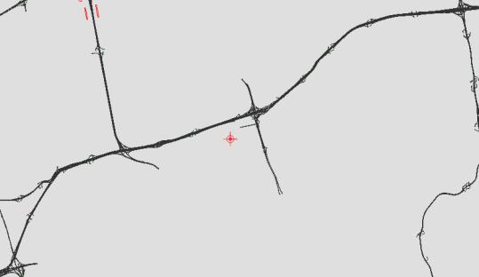
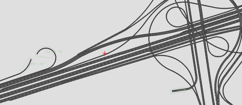
125 Figure 3.3: Toronto 400-Series Highway Microscopic Model 110

126 3.9 Connected Vehicles and RSE Modeling in Paramics By default, Paramics is not capable of modeling real-time information along an entire path to govern the route choice decisions of connected vehicles. In the previous study by the authors [23], a custom plug-in was developed using Paramics API functionality to implement connected vehicle operations and V2V communication. The API records the average speed of each connected vehicle every 5 seconds, and once such a vehicle enters a segment covered by an RSE unit, its average speed is transmitted to the RSE. Connected vehicles were distributed throughout the network based on assumptions of different market penetration rates of such vehicles in the population. The market penetration rates that were considered were 5, 15, 25, 50, 75 and 100 percent. A sensitivity analysis was conducted to assess the influence of the penetration rate on the number and locations of RSE units and the performance of the developed approach. Additionally, beacon objects were implemented to mimic the RSE units in the simulation. In Paramics, beacons are predefined objects that represent points along roadways where information can be delivered to drivers. They have no default functionalities; therefore, in this study, API functions were used to define the mechanism of connectivity between vehicles and the infrastructure. Paramics was used to generate spot speeds for the RSE units, which were employed to calculate the travel times over each entire corresponding CS. In this study, it was assumed that a maximum of 30 snapshots could be saved in the OBD of a connected vehicle. Based on the SAE J2735 standard [35], periodic snapshots were regularly generated at 20-second intervals for vehicle speeds greater than 100 kph and at 6-second intervals for vehicle speeds less than 30 kph. For speeds between 30 and 100 kph, linear interpolation was 111

127 employed to determine the interval of the generated snapshots. When a vehicle was not moving for 5 seconds of a 15-second period, a stop snapshot was recorded and the periodic recording of snapshots was terminated. An API was developed to collect simulated data for connected vehicles based on the scheme described above. The estimated travel times were then compared with the simulated travel times extracted from Paramics. RSE stores both static and dynamic information, such as its communication range and a list of links on which communication is possible. In this study, it was assumed that the range of communication for each RSE unit was 500 meters. The dynamic parameters include the speeds recorded by enabled vehicles and the corresponding timestamps. To avoid excess computational complexity, the communication range of each RSE unit was determined using a simple radial distance criterion. All connected vehicles within the defined range were considered capable of communicating with the RSE unit. If a vehicle could communicate with more than one RSE unit from a given location, the closest was selected. The average speed of the vehicle over the last 5 minutes was calculated and transmitted when that vehicle entered the coverage range of the RSE unit. To consider connectivity among vehicles, information about all other vehicles within the range of the communicating vehicle (within range of the RSE unit) during the last five minutes was also transmitted to the RSE. It should be noted that the travel time estimation for an entire segment is derived through the aggregation of information on the sub-segments covered by RSE units. The average travel time on a sub-segment covered by a given RSE unit is calculated by dividing the length of that sub-segment by the average recorded speed. In other words, one of the advantages of the developed approach compared with other methods, such as those that 112

128 obtain traffic information through Bluetooth or AVI, is that not all connected vehicles are required to travel the entire segment Results As stated above, a 125-km segment of Highway 401 of the 400-series highway network in the GTA was used as the testbed for this simulation study. The average annual daily traffic on this segment is approximately 318,000 vehiclesτ day, and several bottlenecks form along the highway during rush hour, particularly at merging and diverging points. NSGA- II was used as the optimization algorithm to find the optimal number and locations of RSE units to minimize the travel time estimation error with respect to the market penetration of connected vehicles. The detailed NSGA-II results for the optimal placement of RSE units along the highway segment when the market penetration of connected vehicles is 25% are shown in Figures 3.4 to 3.7. Figure 3.8 shows the results for various market penetration rates in the form of the Pareto fronts. The horizontal axis represents the number of RSE units (NR in equation 9), and the vertical axis represents the travel time estimation error (ε in equation 11). The Pareto-optimal set comprises solutions that are not dominated by other solutions. These solutions indicate the best possible compromises with respect to the competing objectives of minimizing the number of RSE units and minimizing the travel time error. Figure 4 shows the Pareto front generated by the multi-objective optimizer for the RSE location problem. As discussed in the formulation section, the highway segment was divided into 250 discrete cells, where each cell represents a potential RSE placement location. The value of each cell can be either 0 or 1, where 1 indicates the presence of an RSE unit at that location and 0 indicates no RSE deployment at that location. The algorithm 113

129 attempts to simultaneously minimize the travel time error (equation 9) and the number of RSE units n to find a solution that provides the optimal number and locations of RSE units. The Pareto solution obtained after 400 generations indicates that the smallest possible number of RSE units is 67 (resulting in a 3% travel time estimation error) and the maximum number is 81 (resulting in a 2% error); these results imply that additional RSE units may not significantly improve the travel time estimation. Because of the stochastic nature of microsimulation models, the simulation model was run with 20 different seed numbers for each RSE configuration. Each seed corresponds to a different random experiment, which may be interpreted as representing a different day in real life. Figure 3.5 depicts the spatial distribution of RSE units along the 125-km segment of Highway 401 considered in the simulation testbed. A comparison of the distributions of RSE and congestion indicates a correlation between the level of congestion and the RSE density; that is, the density of RSE units should be higher in congested regions of a corridor. To quantify this correlation, we used a congestion index [39], defines as the average speed on the segment divided by the free-flow speed for every 1 km of highway, and compared it with the corresponding RSE density (number of RSE units per km). The Pearson's product-moment correlation (PPMC) coefficient was calculated to assess the relationship between the spacing between RSE units and the congestion index. A strong positive correlation was identified, with r(65) =.933 and p <.0005 (Figure 6). A comparison of the correlation index with the critical value and the p-value confirm the significance of the test. The higher RSE density in congested segments can be explained by the fact that in congested segments, the number of snapshots stored on a vehicle s OBD is larger than in 114

130 Travel Time Estimation Error (%) free-flow segments and because of memory constraints, more RSE units are necessary to capture the traffic information from the vehicles. Additionally, in free-flow segments, the travel times between 2 consecutive RSE locations are shorter than those in congested segments, meaning that more RSE units are necessary in congested segments to enable precise estimation of the travel times throughout a traffic jam. Number of RSE Units Figure 3.4: Multi-Objective Optimization Output (Pareto Front) 115

131 Congestion RSE Placement Figure 3.5: Traffic Conditions and Locations for RSE Placement r(65) =.933 p <.0005 Congestion Index Spacing Spacing Between RSEs RSE (Km) Units (km) 3.0 Figure 3.6: Correlation Between RSE Spacing and Congestion Index 116

132 For further examination of the spatial distribution of RSE units, Figure 3.7 presents a histogram of the RSE spacing. The results indicate that the majority of RSE units are spaced 1.5 km apart, with a wide distribution ranging from as close as 0.5 km (in only one case) to as far as 3.0 km (in 4 cases). NSGA-II is a stochastic evolutionary multi-objective algorithm with random elements in the initialization, selection and reproduction steps. Therefore, the optimization result is not always the same. Thus, it is important to perform several runs of the algorithm and conduct a statistical analysis of the results to obtain more robust conclusions. In this study, the model was run 50 times with different crossover and mutation rates (Group 1 to 5), and a hypervolume indicator [40] was calculated to measure the performance of the algorithm. ANOVA statistical testing was also performed to evaluate the mean values of the hypervolume indicator for the different groups of runs. Table 3.1 reports the hypervolume indicator for each run and the ANOVA results. Table 3.1: Sample means of the hypervolume indicator Test Group 1 Group 1 Group 1 Group 1 Group 1 Number Average

133 SUMMARY Groups Count Sum Average Variance Column Column Column Column Column ANOVA Source of Variation SS df MS F p-value F crit Between Groups Within Groups Total The ANOVA test results (p-value > 0.05) for the hypervolume indicator show no significant difference among the results in terms of the number and locations of RSE units, indicating that the algorithm produced stable results. 118

134 Frequency Frequency Spacing Spacing Between Between RSE RSEs Units (Km) (km) Figure 3.7: Histogram of the Distances between RSE Units 3.11 Sensitivity Analysis The influence of the market penetration rate of connected vehicles on the performance of the developed approach was evaluated because the vehicle population is expected to reflect only lower levels of market penetration during the early stages of deployment of this technology. The market penetration rate is defined as the ratio of the number of connected vehicles to the total number of vehicles. This evaluation examined the relationship between the market penetration rate and the number of RSE units required. Market penetration rates of 5, 15, 25, 50, 75 and 100 percent were considered. At each penetration level, the optimization process was applied to identify the optimal number and locations of RSE 119

135 Travel Time Estimation Error (%) units. Figures 3.8 and 3.9 show the relationship between market penetration and the Pareto front of optimal solutions. Market Penetration Number of RSE Units Figure 3.8: Number of RSE Units vs. Market Penetration 120

136 Congestion Index Market Penetration Spacing Between RSE Units (km) Figure 3.9: Spacing Between RSE Units vs. Market Penetration The following conclusions can be drawn from the sensitivity analysis: First, the developed approach demonstrates effective performance in determining the optimal number and locations of RSE units under varying market penetration. Second, increasing the market penetration of connected vehicles results in a reduction in the number of RSE units required along with an improvement in the precision of travel time estimation. These findings can be explained by the fact that when more connected vehicles are available to store, carry and transmit traffic information, fewer RSE units are required to capture the state of traffic along a highway. Finally, the magnitude of improvement is greater for the increase in penetration from 5 to 25 percent than for the increase from 25 to 100 percent, 121

137 indicating a non-linear relationship between the number and locations of RSE units, the precision of travel time estimation and the market penetration of connected vehicles Summary and Conclusion In this paper, a methodology was developed for optimizing the number and locations of roadside equipment (RSE) units for travel time estimation in a vehicle-to-infrastructure (V2I) and vehicle-to-vehicle (V2V) communication environment. The Non-dominated Sorting Genetic Algorithm II (NSGA-II) was used to produce a Pareto front of optimal solutions representing the best possible compromises for simultaneously minimizing the travel time error and the number and locations of RSE units (Figure 3.4). Simulation results from a case study of a 125-km segment of Highway 401 in Southern Ontario show that the accuracy of travel time estimation is, as expected, a function of the optimized RSE placement. The Pareto front (Figure 3.4) shows that the error value is higher when only a few RSE units are placed, and as the extent of deployment increases, the error decreases. After the placement of approximately 81 RSE units at strategic locations, any further increase in the number of RSE units will not significantly reduce the error. The optimal placement of 67 RSE units results in accurate estimates of travel time. The corresponding locations of these 67 RSE units can be obtained from the output of the optimization program, as defined by binary variables (a value of 0 indicates no RSE unit at the corresponding location, and a value of 1 indicates that an RSE unit is deployed at that location). It was found that congested segments require closer RSE placement, which can be attributed to the potential reduction in traffic speeds at bottlenecks. 122

138 In a comparison of the RSE distribution with the level of congestion, Figure 6 indicates a direct correlation between the level of congestion and the RSE density. This figure shows that the RSE density should be higher in congested regions of a corridor, whereas a lower density is more suitable for non-congested sections. This finding is attributed to the datacapturing mechanism used in the connected vehicle environment, which is a function of vehicle speed and congestion. These results suggest that a certain set of RSE locations may exist that will provide better travel time estimates than other placements. Because the associated infrastructure cost is proportional to the number of installed RSE units, a higher RSE density is not always feasible and does not always produce better results. A sensitivity analysis was performed to investigate the effect of the market penetration rate of connected vehicles on the optimal number and locations of RSE units and the travel time estimation error. Six different market penetration rates of 5, 15, 25, 50, 75 and 100 percent were examined for this purpose. The findings confirm the positive impacts of increased market penetration on reducing the number of RSE units required and improving the accuracy of travel time estimation. Notably, the improvement observed for an increase in market penetration from 5 to 25 percent is higher than that for the increase from 25 to 100 percent. The results of this study can be employed by ministries of transportation and other traffic agencies to leverage the application of connected vehicles to reduce the existing number of loop detectors. This may reduce capital expenditure, operations, and maintenance costs and facilitate the provision of accurate real-time information to drivers. 123

139 Although the proposed approach shows promising results, several limitations must be addressed in future research. In this study, the communication between individual vehicles and between vehicles and the surrounding infrastructure was assumed to be perfect, with no communication delays or packet drops, which is unlikely in the real world. The assumption of a deterministic read range also requires further investigation based on the non-deterministic characteristics of such a network. Therefore, in future research, the explicit modeling of wireless communications must be examined in greater depth and with due consideration for uncertainties. In addition, the influence of non-recurring types of congestion, such as collisions, along with the impacts of collecting and augmenting traffic information from other sources, such as smartphones, must be examined in future work. 124

140 REFERENCES [1] Liu, Henry X., Xiaozheng He, and Will Recker, "Estimation of the timedependency of values of travel time and its reliability from loop detector data," Transportation Research Part B, no. 4, pp , [2] Petty, Karl F., et al, "Accurate estimation of travel times from single-loop detectors," Transportation Research Part A, vol. 32, no. 1, pp. 1-17, [3] D. Bremmer, K. Cotton, D. Cotey, and C. Prestrud, "Measuring congestion: learning from operational data," Transportation Research Record, no. 1895, pp , [4] Omrani, R., Izadpanah, P., Nikolic, G., Hellinga, B., Hadayeghi, A., & Abdelgawad, H, "Evaluation of wide-area traffic monitoring technologies for travel time studies," Journal of the Transportation Research Board, vol. 2380, pp , [5] Calabrese, F., M. Colonna, P. Lovisolo, D. Parata, and C. Ratti, "Real-Time urban monitoring using cellphone: A case study in Rome," IEEE Transactions on intelligent Transportation System, vol. 12, no. 1, pp , [6] Herrera, J. C., D. B. Work, R. Herring, X. Ban, Q. Jacobson, and A. M. Bayen, "Evaluation of Traffic Data Obtained via GPS-enabled Mobile Phones: the mobile Century Field Experiment," Transportation Research Part C: Emerging Technologies, vol. 18, no. 4, pp , [7] Coifman, B., and M. Cassidy, "Vehicle Reidentification and Travel Time Measurement on Congested Freeways," Transportation Research Part A: Policy and Practice, vol. 36, no. 10, pp , [8] Dion, F., and H. Rakha, "Estimating Dynamic Roadway Travel Times Using Automatic Vehicle Identification Data For Low Sampling Rates," Transportation Research Part B: Methodological, vol. 40, no. 9, p , [9] Faouzi, N.E.El., R. Billot, S. Bouzebda, "Motorway Travel Time Prediction Based on Toll Data and Weather Effect Integration," IET Intelligent Transport Systems, vol. 4, no. 4, pp ,

141 [10] Click, S. M., and T. Lloyd, "Click, S. M., and T. Lloyd. Applicability of Bluetooth Data Collection Methods for Collecting Traffic Operations Data on Rural Freeways," in TRB 91st Annual Meeting, Washington, [11] Haseman, R. J., J. S. Wasson, and D. M. Bullock, "Real-Time Measurement of Travel Time Delay in Work Zones and Evaluation Metrics Using Bluetooth Probe Tracking," Transportation Research Record: Journal of the Transportation Research Board, no. 2169, p , [12] C.S. ReVelle, and Eiselt, H.A, "Location analysis: a synthesis and survey," European Journal of Operational Research, vol. 165, pp. 1-19, [13] S. Chan, and H.K. Lam, "Optimal speed detector density for the network with travel time information," Transportation Research A, vol. 36, pp , [14] A. Ehlert, M. Bell, and S. Grosso, "The optimization of traffic count locations in road networks," Transportation Research Record, Part B, vol. 40, pp , [15] Sherali, H.D., J. Desai, and H. A. Rakha, " Discrete Optimization Approach for Locating Automatic Vehicle Identification Readers for the Provision of Roadway Travel Times," Transportation Research Part B: Methodological, vol. 40, no. 10, pp , [16] H. a. J. Z. Yang, "Optimal Traffic Counting Locations for Origin-Destination Matrix Estimation," Transportation Research Part B: Methodological, vol. 32, no. 2, pp , [17] Ehlert, A., M. Bell, and S. Grosso, "The Optimization of Traffic Count Locations in Road Networks," Transportation Research Part B: Methodological, vol. 40, no. 6, pp , [18] Kwong, K., R. Kavaler, R. Rajagopal, and P. Varaiya, "Arterial Travel Time Estimation Based on Vehicle Re-identification Using Wireless Magnetic Sensors," Transportation Research Part C: Emerging Technologies, vol. 17, no. 6, pp , [19] A. Sen, P. Thankuriah, X. Zhu, and A. Karr, "Frequency of probe reports and variance of travel time estimates," Journal of Transportation Engineering, vol. 123, no. 4, pp ,

142 [20] K. Ozbay, B. Bartin, and S. Chien, " South Jersey real-time motorist information system: technology and practice," Transportation Research Record, Transportation Research Board of the National Academies, no. 1886, pp , [21] B. Bartin, K. Ozbay, and C. Iyigun, "A clustering based methodology for determining the optimal roadway configuration of detectors for travel time estimation," Transportation Research Record, Transportation Research Board National Research Council, no. 2000, pp , [22] Kianfar, Jalil, and Praveen Edara, "Placement of Roadside Equipment in Connected Vehicle Environment for Travel Time Estimation," Transportation Research Record: Journal of the Transportation Research Board, vol. 2381, pp , [23] Olia, Arash, Abdelgawad, Hossam, Abdulhai, Baher, Razavi, Saiedeh N., "Assessing the Potential Impacts of Connected Vehicles: Mobility, Environmental and Safety Perspectives," Journal of Intelligent Transportation Systems: Technology, Planning, and Operations, no , [24] Xu, H., and M. Barth, "Travel Time Estimation Techniques for Traffic Information Systems Based on Intervehicle Communications," Transportation Research Record: Journal of the Transportation Research Board, vol. 1944, p , [25] Rim, H., Oh, C., Kang, K., & Kim, S, "Estimation of lane-level travel times in vehicle-to-vehicle and vehicle-to-infrastructure-based traffic information system," Transportation Research Record: Journal of the Transportation Research Board, vol. 2243, pp. 9-16, [26] Oh, C., T. Kim, W. Kim, S. Hong, and J. Park, "Capability-Enhanced Probe Vehicle Surveillance System with Vehicle-to-Vehicle Communications: Framework and Evaluation," Transportation Research Record: Journal of the Transportation Research Board, no. 2189, pp. 8-16, [27] D. E. Goldberg, Genetic Algorithms in Search, Optimization and Machine Learning, 1-32: Reading, MA: Addison-Wesley, [28] a. R. C. M. Gen, Genetic Algorithms & Engineering Optimization, New York: John Wiley and Sons, [29] P. Edara, J. Guo, B. L. Smith, and C. McGhee, "Optimal placement of point detectors on Virginia s freeways: case studies of northern Virginia and Richmond," Virginia Transportation Research Council, Virginia,

143 [30] E. Zitzler, "Evolutionary algorithms for multiobjective optimization: Methods and applications.," Ithaca: Shaker, [31] Corne, David W., Joshua D. Knowles, and Martin J. Oates, "The Pareto envelopebased selection algorithm for multiobjective optimization," in Parallel Problem Solving from Nature PPSN VI, Springer Berlin Heidelberg, 2000, [32] N. Srinivas, K. Deb., "Multi-objective function optimization using nondominated sorting genetic algorithms," Evolutionary Computation, vol. 2, no. 3, pp , [33] Deb, K., Pratap, A., Agrawal, S. and Meyarivan, T, "A fast and elitist multiobjective genetic algorithm: NSGA-II," Evolutionary Computation, IEEE Transactions on, vol. 6, no. 2, pp , [34] Ghiasi, Hossein, Damiano Pasini, and Larry Lessard, "A non-dominated sorting hybrid algorithm for multi-objective optimization of engineering problems," Engineering Optimization, vol. 43, no. 1, pp , [35] SAE-International, "DSRC Implementation Guide: A guide to users of SAE J2735 message sets over DSRC," DSRC Committee, [36] P. Edara, J. Guo, B. L. Smith, and C. McGhee, "Optimal placement of point detectors on Virginia s freeways: case studies of northern Virginia and Richmond," Virginia Transportation Research Council, Virginia Department of Transportation, [37] Patil V.P. and Pawar D.D., "The optimal crossover or mutation rates in genetic algorithm : A review," International Journal of Applied Engineering and Technology, vol. 3, pp , [38] Abdelgawad, H., Abdulhai, B., Amirjamshidi, G., Wahba, M., Woudsma, C., & Roorda, M. J, "Simulation of exclusive truck facilities on urban freeways," Journal of transportation engineering, [39] T. J. Lomax, Quantifying congestion, Transportation Research Board, 398, [40] Zitzler, E., Thiele, L., Laumanns, M., Fonseca, C. M., & Da Fonseca, V. G., "Performance assessment of multiobjective optimizers: an analysis and review," Evolutionary Computation, IEEE Transactions on, vol. 7, no. 2, pp ,

144 CHAPTER 4: FULLY AUTOMATED VEHICLES: A STUDY OF FREEWAY TRAFFIC FLOW This chapter is based on the following submitted journal paper: Olia, A., Razavi, S.N. (2016). Fully Automated Vehicles: A Study of Freeway Traffic Flow, Journal of Intelligent Transportation Systems, submitted in March Fully automated vehicles (AVs) are already being road tested and will be publicly available in the near future. Whereas vehicles that are currently available on the market include a variety of semi-automated functions, such as adaptive cruise control and collision avoidance, AVs require no driver intervention and perform all driving functions for an entire trip. According to a review of the literature, many studies have been conducted on the influence of semi-automated functions such as adaptive cruise control; however, to our knowledge, evaluations of the impacts of AVs under realistic conditions are rare. To this end, we further divide AVs into two categories: cooperative and autonomous. Both cooperative and autonomous AVs are driverless vehicles. These two classes of AVs can be distinguished based on the nature of their connectivity and the role it plays in their technology, as follows: an autonomous AV depends only on the information that can be sensed by the vehicle itself through lidar, radar or video image processing, whereas a cooperative AV supplements the information it receives from sensors with information obtained through vehicle-to-vehicle (V2V) communication. Although the primary motivation for the adoption of AVs is safety and comfort, they can also improve highway capacity, especially at high market penetration. However, few studies have addressed the capacity implications of AVs under realistic conditions, such as driving in mixed traffic or lane merging with AVs at a market penetration of less than 100%. In doing so, this paper evaluates and examines the effect of AV technologies on traffic flow behavior and the resulting improvements in highway capacity. To this end, a car-following and lane-merging model based on the Fritzsche model is developed for AVs and implemented in a microsimulation model. Given the limitations of microsimulation models, the default carfollowing and lane-merging models are overridden and extended to realistically simulate the behaviors of AVs. This model is implemented for a segment of a highway that includes an on-ramp in a microsimulation environment. The results indicate that a maximum lane capacity of 6,450 vph is achievable if all vehicles are cooperative AVs. The introduction of cooperative AVs at a low market penetration (less than 30%), as expected, results in the least capacity benefits; in this case, the vehicles are scattered across all lanes of a multilane highway and thus lack frequent opportunities for one cooperative AV to follow another cooperative AV. By contrast, with the incorporation of autonomous AVs into the traffic 129

145 stream, the achievable capacity is highly insensitive to market penetration; the capacity remains within a narrow range of 2,046 to 2,238 vph regardless of market penetration. As a result, it can be concluded that autonomous vehicles, even at high market penetration, can have only a small impact on highway capacity. Based on these premises, this research is focused on quantifying the potential benefits of AVs to provide insight into how these technologies will impact road users and network performance. To conclude, the results of this study demonstrate the significance of communication in achieving the benefits offered by cooperative AVs. 130

146 4.1 Abstract As a result of recent developments in the field of vehicle automation, intelligence and communication systems, automated vehicles have begun to receive tremendous interest among researchers and decision-makers because of their substantial safety and mobility benefits. It is expected that these technologies will fundamentally change the way traffic flows through our road networks in the near future. Although much research has been reported regarding the implications of Adaptive Cruise Control (ACC) and Cooperative Adaptive Cruise Control (CACC) technologies for highway capacity, to our knowledge, evaluations of the impacts of automated vehicles (AVs) are rare. AVs can be divided into two categories, cooperative and autonomous. Cooperative AVs, unlike autonomous AVs, can communicate with other vehicles and infrastructure, thereby providing better sensing and anticipation of preceding vehicles actions, which would have an impact on traffic flow characteristics. This paper proposes a methodology for quantifying and evaluating the impacts of AVs on the capacities of highway systems. To achieve this goal, a model incorporating the impacts of AVs technology on car-following and lane-merging behavior is formulated, based on which an estimate of the achievable capacity is derived. A microsimulation study is performed to evaluate and verify the model, and an example is provided to demonstrate an application of the methodology. To consider the period before AVs account for a majority of the vehicles in traffic networks, the proposed model considers combinations of vehicles with varying market penetration. The results indicate that a maximum lane capacity of 6,450 vph (300% improvement) is achievable if all vehicles are driven in a cooperative automated manner. Regarding the incorporation of 131

147 autonomous AVs into the traffic stream, the achievable capacity appears highly insensitive to market penetration, namely, the capacity remains within a narrow range of 2,046 to 2,238 vph irrespective of market penetration. It can be concluded that autonomous AVs cannot improve capacity and that their behavior is highly similar to that of regular vehicles. The results of this research provide practitioners and decision-makers with knowledge regarding the potential capacity benefits of AVs with respect to market penetration and fleet conversion. 132

148 4.2 Introduction Traffic congestion continues to increase in metropolitan areas, contributing to billions of dollars of losses due to congestion [1]. Traffic congestion may occur for one or a combination of the following two reasons: 1) an increase in demand (number of people or trips in the transportation system) or 2) a decrease in the supply or capacity of the transportation system (roadway network or public transit network). With the limited budgets and financial and societal constraints facing major cities, infrastructure expansion is becoming financially infeasible and unsustainable [2]. Recent advances in information and communication technology (ICT) offer myriad opportunities to enhance the operations of existing transportation networks without the need to physically expand them or build more roads. These advances can enhance the efficiency and reliability of transportation systems and improve all aspects of drivers decision-making processes, from operational to strategic decisions. At the operational level, these technologies can help drivers and vehicles make safe and reliable decisions concerning lane changes, acceleration, and deceleration. Automated and human-driven vehicles behave in accordance with different types of driving logic: 1) humans have longer reaction times than computers do, and 2) humans must consider more decision variables to overcome the uncertainty associated with human decision-making processes. Consequently, gap acceptance and car-following behavior have been extensively evaluated in the literature [3-8], and different models with varying levels of complexity have been introduced to capture the underlying decision-making processes for gap acceptance and acceleration [9-14]. Despite these contributions, many of these studies have not modeled 133

149 the behavior of automated vehicles (AVs) navigating through transportation networks and the literature that strives to capture such behavior is rather limited. AVs may be partially automated, offering driver assistance functionalities, or fully automated, requiring no driver intervention. Fully AVs can be further divided into two categories: cooperative and autonomous. Both cooperative and autonomous AVs are driverless vehicles. Autonomous AVs depend only on the information that can be sensed by the vehicle through lidar, radar or video image processing, whereas cooperative AVs augment the information they receive from sensors with information obtained through vehicle-to-vehicle (V2V) communication. Autonomous AVs aspire to eliminate human driving altogether (driverless cars), increasing the convenience and utility of cars and potentially enhancing safety by eliminating human error. An autonomous AV would sense its environment and navigate through it without a driver and without input from other vehicles or the infrastructure. By contrast, cooperative AVs aspire to extremely rapid reactions to their environments, such as the use of dedicated short-range communications (DSRC) to communicate with other vehicles or infrastructure. However, autonomous operation may require larger inter-vehicular spacing and headways and may decrease road capacity, or at least not increase it, as in the case of cooperative vehicles. Figure 4.1 summarizes the processes of sensing and communication performed by AVs. 134

150 Measuring the range and rate via radar, lidar or video processing (a) Autonomous Automated Vehicles Receiving acceleration information directly through communication (b) Cooperative Automated Vehicles Figure 4.1: Cooperative and Autonomous Automated Vehicles Early attempts to model driving environments with AVs focused primarily on automated highway systems (AHSs), in which fully autonomous vehicles operate in a set of dedicated lanes [15-20]. Implementing an AHS is costly and requires a large fleet of fully autonomous vehicles to be efficient; therefore, such systems have never been fully implemented or realized. Instead, the AHS concept has evolved into the concept of driver assistance systems. Primitive versions of driver assistance systems, such as adaptive cruise control (ACC), which adjusts a vehicle s speed based on the leader s speed, rely solely on on-board sensors [21-24]. ACC-enabled vehicles are an advanced version of conventional cruisecontrol enabled vehicles. ACC strives to maintain the speed originally set by the driver. However, ACC is able to detect the range (distance) and the rate of change of this range (speed) of the preceding vehicle. ACC consequently enables a vehicle to decelerate or accelerate depending on the behavior of the vehicle in front. 135

151 Connectivity among vehicles and the infrastructure (both V2V and vehicle-to-infrastructure (V2I) connectivity) improves the performance of driver assistance systems [25-28]. For example, an ACC system can use information from V2V communication networks to automatically adjust a vehicle s speed based on the speed of the leading vehicle more rapidly than conventional ACC vehicles can. This new type of system is called cooperative adaptive cruise control (CACC). Various acceleration algorithms have been proposed in the literature for controlling vehicles with CACC. Arem et al. [29] proposed a car-following logic for CACC that uses relative speed, safe deceleration, current acceleration, and spacing with respect to the immediate leader to calculate the acceleration at the next decision point. Wang et al. [30] proposed a CACC algorithm based on a model predictive control process in which each vehicle uses information from its leader to predict the platoon s behavior. In [31], a CACC system that allows for communication between vehicles was examined in a network incorporating different types of vehicles, including manually operated vehicles, ACC vehicles, and CACC vehicles, with varying market penetrations. The results showed that ACC and CACC vehicles increased highway capacity by 11% and 200%, respectively. Shladover et al. [32] examined the potential increase in network throughput at different CACC market penetration rates. Their results showed that a maximum lane capacity of approximately 4,000 vph could be achieved if all vehicles were equipped with CACC. Milanes et al. [33] investigated the performance of CACC in a field trial using 4 vehicles equipped with CACC and DSRC devices to exchange information. Their study revealed that CACC could improve the response time of a following vehicle to any change in the speed of the leading vehicle, thereby improving stability with respect to inter-vehicular 136

152 spacing (also known as string stability). Another CACC field trial, the Connect & Drive project [34], demonstrated that a platoon of vehicles using CACC with a time headway of 0.7 s could result in string stability. Michel et al. [35] calculated the capacity of an AHS and found a capacity of 7,000 vph per lane with 100% AVs. Carbaugh et al. [36] considered the safety implications of AVs compared with manual driving. Their model yielded the probability distribution and severity of the first rear-ends crash caused by a hard braking disturbance on the highway. Their model indicated that at a given speed and capacity, the probability of collision with AVs is between 30% and 90% lower, depending on the relative velocity at collision. The USDOT s definition of AVs is rather general and includes five different levels of automation [37], as follows: - Level 1: no automation; refers to regular vehicles, as defined previously, for which drivers are the only decision-makers. - Level 2: function-specific automation; refers to vehicles with at least one vehicle control function. Electronic stability control and lane adjustment are two examples of such control functions. - Level 3: combined function automation; refers to vehicles with at least two vehicle control functions. These control functions operate in unison and provide additional assistance to the driver. - Level 4: limited self-driving automation; refers to vehicles that can control safetycritical functions. However, their ability is limited to certain weather, roadway, and 137

153 traffic conditions. The driver can resume control of the vehicle if necessary, and sufficient time is provided for this transition. - Level 5: full self-driving automation; refers to fully automated vehicles. A vehicle with this level of automation controls all driving functions under all weather, road, and traffic conditions. To estimate the effectiveness of autonomous vehicles under mixed traffic conditions and in non-platooning states, a number of field trials have been performed, including Safe Road Trains for the Environment (SARTRE) and Europe s KONVOI system [38, 39], and a number of concepts, such as non-platooning autonomous vehicles, including the Google Car [40], have been explored. These initiatives have significantly advanced the research and development in this field, with a primary focus on safety as well as environmental and comfort benefits. Nowakowski et al. [41] examined driver acceptance gaps of less than 1 s, finding that drivers were generally comfortable with and typically selected the following time gaps of less than 1 s offered by the CACC system. Drivers willingness to accept shorter following gaps adds credibility to the assertion that future CACC systems may have the potential to significantly increase the achievable capacity of highway lanes. Based on the statistical analysis presented in [42], the desired time gap that human drivers will maintain with a preceding vehicle is normally distributed, with a mean of 1.1 s and standard deviation of 0.15 s. In [43, 44, 45 and 46], the desired time gaps of ACC and CACC vehicles were evaluated based on field tests and identified as 1.1 s and 0.6 s, respectively. It should be noted that for reasons of safety and string stability, ACC systems should not be designed to operate with time gaps of less than 1.0 s [47]. 138

154 Lane merging is one of the major factors that contributes to degrading the capacity of a road system under congested conditions [48, 49, 50 and 51]. Drivers must check the available gap with respect to the vehicle in front and the following vehicle in the target lane to perform a merging maneuver. Given the limitations of human drivers, these sets of synchronized perceptions and actions decrease the efficiency and safety of merging into the mainline, which consequently triggers speed breakdown and shockwave effects. Cooperative and autonomous AVs are expected to improve the efficiency and safety of lane-merging maneuvers by means of their own control systems and their ability to sense and interact with the infrastructure and other vehicles. The most conventional strategy for preventing the mainline of a highway from becoming over-congested and maximizing capacity efficiency is to use ramp metering to restrict the rate at which on-ramp vehicles enter the mainline. However, ramp-metering strategies have been found to be effective only at high levels of demand and when the ramps are close together [52]. According to a literature review, various algorithms have been suggested for managing merging maneuvers with different levels of automation at the vehicle level. In [53], a merging algorithm for a one-lane AHS was introduced in which a merging vehicle enters the mainline only if there is an available gap. Autonomous merging was also evaluated in [54], based on a control algorithm developed for autonomous vehicles driving on a highway with multiple merge junctions. In [55 to 61], various strategies and algorithms were developed to evaluate the effects of AVs and communication on the merging process. To our knowledge, most research on lane merging has been conducted based on the assumption that all vehicles are automated and able to communicate with other vehicles and the 139

155 infrastructure, that is, it is assumed that the market penetration of AVs is 100%. However, this assumption is not achievable in the near future. A more realistic scenario would involve mixed traffic of both automated and regular vehicles. From the literature review presented above, it can be concluded that much work has been reported regarding specific and limited applications of automation in vehicles, such as ACC or CACC, and these studies emphasize the positive impacts of such technologies in improving highways capacity. However, previous studies have not examined the role of fully AVs under mixed traffic conditions and have been confined to specific scenarios, such as the longitudinal control of vehicle motion. In other words, the effects of AVs on road capacity have been reported only for basic segments of highway, without considering the disturbances caused by merging, weaving and diverging maneuvers around ramps, and only at high levels of market penetration. To close this gap, this paper proposes a methodology for evaluating and quantifying the benefits and efficacy of cooperative and autonomous AVs in improving highway capacity. To this end, a model incorporating the impacts of AVs technologies on car-following and lane-merging behavior is formulated, based on which an estimate of the achievable capacity is derived. A microsimulation study is performed to evaluate and verify the model, and an example is provided to demonstrate an application of the methodology. To consider the period before AVs account for a majority of the vehicles in traffic networks, the proposed model considers a combination of vehicles with varying market penetration. The results of this research provide practitioners and decision-makers with information concerning the mobility benefits of AVs with respect to market penetration and fleet conversion. 140

156 The remainder of this paper is organized as follows. In Sections 2 and 3, a car-following model for human drivers and the Fritzsche model are discussed. Then, in Section 4, a carfollowing model for AVs and their impacts is incorporated into the modeling of driving behavior. In Section 5, the proposed automated merging model for the on-ramp merging of AVs is explained. Microsimulation and statistical analysis performed in section 6 and 7. Finally, the findings and results are summarized at the end of the paper. 4.3 Car-Following Model for Regular Vehicles We introduce three types of vehicles into our model to consider all possible combinations: 1. Regular vehicles. The drivers car-following and lane-changing behavior is governed by Fritzsche s model [62], which incorporates the Wiedemann [63] carfollowing algorithm. 2. Autonomous AVs. For this type of vehicle, car following is determined based on a simple first-order control law representing gentle responses to changes made by the car ahead. 3. Cooperative AVs. This type of vehicle, using V2V communications, allows closer vehicle following when following another cooperative AV. If it is following a manual vehicle or an autonomous AV, it behaves similarly to an autonomous AV. The automated car-following capability enables faster responses to changes made by the car ahead and permits following at significantly shorter time gaps, based on the gap values chosen by drivers in a field test [64]. 141

157 Considering the lack of public documentation of the car-following dynamics of real autonomous vehicles, a simple first-order dynamic response for autonomous-vehicle car following was adopted from Fritzsche and Wiedemann s model [62, 62]. The car-following and lane-changing behavior of manual drivers is based on a psychophysical model that was developed by Fritzsche and is used in the PARAMIC [65] microsimulation traffic modeling software. Figure 4.2 illustrates the notations used to describe the Fritzsche car-following model. Direction Vehicle n v n Vehicle n-1 v n-1 x n l n-1 xn-1 Figure 4.2: Car-Following Model Notation X n Position of vehicle n (m) v n Speed of vehicle n (mτ s) x Space headway, x n 1 x n (m) v Difference in speed, v n v n 1 (mτ s) l n Length of vehicle n (m) 142

158 S n 1 Effective length of vehicle (n 1), L n 1 + standstill distance (m) Standstill Distance (m): Distance between Stopped Vehicles 4.4 Fritzsche Car-Following Model The Fritzsche model includes 5 regimes defined based on drivers perceptions of the speed difference between two vehicles. For instance, the speed difference must be of a certain magnitude to be perceived by the driver at all. Fritzsche developed the following regimedefining thresholds. The thresholds for the perception of negative (PTN) and positive (PTP) speed differences are defined in Equations 1 and 2: PTN = K PTN ( X S n 1 ) 2 f x (1) PTP = K PTP ( X S n 1 ) 2 + f x (2) where KPTN, KPTP and fx are model parameters. The following vehicle does not perceive speed differences below the threshold values of PTN and PTP. The Fritzsche model not only accounts for the perception thresholds regarding speed differences but also considers four thresholds regarding the space headway between the following and leading vehicles (Equations 3 8). The desired distance, AD, defines the gap that a driver will strive to maintain with the preceding vehicle and is defined as follows: AD = S n 1 + T D V n (3) where TD is the desired time gap. 143

159 The risky distance, AR, represents the threshold at which the distance headway becomes too close for comfortable driving and is defined as AR = S n 1 + T r V n 1 (4) where Tr is the risky time gap. For gaps smaller than the risky distance, drivers must decelerate heavily to prevent collisions. The safe distance, AS, represents the minimum headway threshold at which positive acceleration is applied if the distance between the leader and the follower is increasing. The safe distance is defined as follows: AS = S n 1 + T s V n (5) where Ts is a model parameter. The braking distance, AB, is limited by a vehicle s maximum deceleration. Therefore, collision is possible when the initial speed difference between two vehicles is large, even if the following vehicles brakes with the maximum deceleration. The available braking distance required to prevent collision is calculated as AB = AR + V2 b m (6) where bm is defined as b m = b min + a n 1 (7) 144

160 bmin and an-1 are the model parameters that control the maximum deceleration required to prevent collision. Danger: The spacing between the vehicles is smaller than the risky distance AR. The following vehicle applies its maximum deceleration, bmin, to extend the gap. Free driving: The follower can accelerate at its maximum acceleration rate to achieve the desired speed. The relationship between the time gaps defined above is as follows: T r < T s < T D (8) Based on the Fritzsche car-following model, a vehicle strives to maintain the gap with respect to the vehicle ahead at a value between the desired spacing (AD) and the risky spacing (AR) to prevent a potential collision (Equations 9 and 10): AD = S g + T D V n (9) AR = S g + T r V n 1 (10) where Sg is the gap between vehicles at traffic jam density and V n and V n 1 are the speeds of the following and leading vehicles, respectively. By merging Equations 9 and 10, the Fritzsche model can be summarized as follows: AD S g V n (t + t) = min T D AR S g, u f (11) { T r 145

161 where u f is defined as the space-mean traffic stream free-flow speed of the highway segment. 4.5 Car-Following Model for Cooperative and Autonomous Automated Vehicles Cooperative and autonomous AVs are able to interact with the vehicles ahead of them and automatically adjust their speed to prevent collisions. To this end, the controller of such a vehicle needs to obtain the trajectory information of the leading vehicle, such as its speed, location, and acceleration. The controller uses sensors to derive this trajectory information. Cooperative AVs, unlike autonomous AVs, participate in direct communication with the vehicles ahead. An autonomous AV can only measure the direct distance to and relative velocity of the preceding vehicle. As a result, the acceleration of the preceding vehicle can only be estimated from this information while a cooperative AV is able to gather the relevant acceleration information as soon as the preceding vehicle accelerates or decelerates. This information not only can be received and processed by cooperative AV faster but also is more accurate. In addition to the desired time gap, another difference between automated and autonomous vehicles is automated merging, which allows a vehicle to merge into the mainline of a highway with the least possible disturbance. The lane-changing and merging behavior of autonomous and regular vehicles is governed by the gap acceptance theory, i.e., every driver has a critical gap for which the lane-merging process can be performed safely. Drivers always compare the existing gap between the preceding and following vehicles in the target lane to the minimum required gap; if the gap satisfies the necessary conditions, 146

162 then the driver will perform the merging maneuver (Equations 12 and 13, known as the Gipps model) [66]: S 1 h V 1 + V 1 D 1 (12) where S 2 h V 2 + V 2 D 2 (13) S n : gap between the vehicle and the vehicle ahead or behind in the target lane V 1 = V 1 V (mτ s) V 2 = V V 2 (mτ s) V 1 : speed of the vehicle ahead in the target lane (mτ s) V 2 : speed of the vehicle behind in the target lane (mτ s) V: speed of the merging vehicle (mτ s) D n : maximum deceleration of vehicle n (m Τ s 2 ) To find a safe gap, it is necessary to meet the conditions introduced in Equations 12 and 13, which could trigger speed breakdown and congestion effects. By contrast, cooperative AVs have access to the exact geometry of the network as well as direct communication (V2V) with other cooperative AVs within range and can exchange information regarding the speeds and positions of leading and following vehicles. Consequently, cooperative AVs can more effectively perform merging maneuvers using the available gaps. The carfollowing and lane-merging algorithm for cooperative and autonomous AVs is explained 147

163 further below. The following variables are used to define the proposed car-following control algorithms for automated and autonomous vehicles: V = Current speed of the AV (m/s) V d = Speed limit of the road (m/s) V f = Speed of the preceding vehicle (m/s) T d = Desired time gap of the AV (s) g = Existing gap (m) g d = Desired gap (m) Cooperative and autonomous AVs follow the same car-following model, albeit with two differences. 1) Cooperative AVs have the ability to communicate and share traffic information via wireless communications (DSRC) or vehicular networks. Because of such direct communication, they can access more accurate trajectory information for their preceding vehicles and can react faster to any change, such as the acceleration or deceleration of a car in front. Consequently, compared with autonomous AVs, cooperative AVs can tolerate smaller time gaps. 2) Cooperative AVs, unlike autonomous or regular vehicles, can better utilize the available gaps between vehicles and more efficiently perform merging maneuvers as a result of coordination and communication. The lane-changing and merging behavior of both regular and autonomous vehicles is governed based on the gap acceptance theory. Specifically, drivers initially evaluate the speeds and positions of the 148

164 following and leading vehicles in the target lane and execute lane changes only if the gap between them is sufficient. The proposed car-following model has two components, namely, speed and gap control, which should control both the speed and gap of an AV simultaneously at each time step in response to any change in the speed or position of the preceding vehicle to prevent collisions. The gap control module checks the gap between the vehicles and attempts to ensure the desired gap between the controlled vehicle and the vehicle ahead of it. The speed control module maintains the vehicle s speed close to the desired speed or the speed limit. Forward-looking sensors on AVs have only a limited range in which they can detect preceding vehicles. A typical range for these sensors is between 100 and 200 m [67-70]. The auto-cruise radar system manufactured by TRW [71] has a forward-looking range of up to 150 m and operates at vehicle speeds ranging from 30 to 180 kph. Delphi s [72] newest generation of electronically scanning radar (ESR) can scan 200 m forward. Google s driverless car is able to detect obstacles up to 200 m away [73]. The Mercedes S- Class autonomous car provides the sensing of objects from a few cm to as much as 200 m away [74]. Nissan s autonomous Leaf car is equipped with forward-looking microwave radar with a 200-m range [75]. Given the range of comfortable and gentle acceleration and deceleration for AVs [47], the impacts of the detection range on the required deceleration are evaluated below, following an explanation of the car-following model algorithm. Based on the Fritzsche car-following model, driver behavior is defined based on 5 regions and 6 thresholds regarding differences in speed and gap lengths, considering both the 149

165 stochastic nature of traffic and the large diversity in space- and time-response characteristics among different drivers. A vehicle will attempt to maintain its gap with respect to the vehicle ahead at a value between the desired spacing (AD) and the risky spacing (AR) to prevent collisions (Equations 9 and 10). The thresholds considered in the Fritzsche car-following model reflect the fact that drivers cannot observe sufficiently small changes in speeds or gaps and do not follow each other at a constant distance. By contrast, compared with human drivers, the observations and actions of AVs are substantially faster and more accurate; consequently, such vehicles follow their preceding vehicles based on their desired time gaps without any oscillation in time headway. The desired gap is assumed to be a linear function of speed. It is defined based on the premise that the desired gap is a characteristic of the AV and not of driver preference. As a result, drivers reaction times are eliminated from the model. The desired gap, g d, and speed difference, d v, are defined in Equations 18 and 19. g d = V T d + S d (18) d v = V V d (19) where S d is the standstill distance. At each time step, an AV measures its existing gap and speed difference with respect to the location and speed of the vehicle ahead. If an AV observes a vehicle within its detection range, the gap control component controls the motion of the vehicle; otherwise, only the speed control component is active. To ensure comfortable and safe operation, the ISO 150

166 15622 standard [47] confines the maximum deceleration and acceleration rates of such a vehicle to -3mΤ s 2, and +2 mτ s 2, respectively. Based on the literature discussed previously, the forward-looking sensors of AVs have a limited range and are typically able to detect barriers and vehicles within a range of 100 to 200 m. To determine the effective sensing range, a sensitivity analysis of the change in speed versus the detection range was performed. For this experiment, we assumed that the distance between consecutive vehicles was greater than 200 m and that the following and preceding vehicles were driving at speeds of 30 and 10 mτ s, respectively. Figure 4.3 presents the change in speed of a following vehicle after it observes a change in the preceding vehicle. The maximum required deceleration rate determined for the following vehicle indicates that when the range is 50 m, the required deceleration rate is not only higher than recommended rate for AVs vehicles but also higher than emergency braking capability of such vehicles, e.g., 0.9g [76, 77 and 78], which is not acceptable from the safety perspective. Moreover, a gradual reduction in speed is more conducive to maintaining smooth traffic flow near a bottleneck. Speed homogenization decreases the required number of deceleration and acceleration maneuvers and, consequently, the number and severity of oscillations in traffic flow [79 and 80]. By contrast, discontinuity between different states of traffic flow on a highway produces shockwaves. The traffic shockwaves caused by an unstable traffic stream are a well-analyzed traffic phenomenon and are known to be a major cause of traffic congestion. Therefore, reducing the likelihood of the formation and propagation of shockwaves through speed homogenization can improve the operational performance of a highway. Consequently, if 151

167 the detection range were to diminish significantly below 100 m, e.g., 50 m, this range reduction would adversely affect vehicle-following performance. 152

168 -1.6 m/s/s Detection range -1.2 m/s/s -2.3 m/s/s -20 m/s/s (a) Autonomous Vehicles -1.8 m/s/s -2.8 m/s/s Detection range -1.1 m/s/s -8 m/s/s (b) Automated Vehicles Figure 4.3: Impact of Detection Range on Deceleration rate 153

169 The impact of the detection range of preceding vehicle on highway capacity is evaluated and illustrated below. Based on the above discussions, the detection range threshold was selected to be 150 m. In other words, if the leading vehicle is farther than 150 m away in this model, the AV does not account for the vehicle ahead and therefore applies only speed control (Equation 19). If the distance to the preceding vehicle is 150 m or less, it applies automatic spacing control (Equation 18). If the existing gap is smaller than the desired gap threshold defined in Equation 18, then to prevent collisions, the maximum emergency deceleration rate of 8 m s2 [81] is applied by the AVs, as represented in Equation 20: if g < g d then a = a max m s 2 (20) When the spacing between the vehicles is greater than 150 m, namely, the threshold between the activation of the gap and speed control components, the acceleration and deceleration applied to the vehicle are functions only of the difference between its desired and current speeds. Equation 21 defines the behavior of a vehicle under these conditions. This equation ensures that the applied acceleration and deceleration rates will lie within the range of -3 m to 2 m s 2 s2. The comfortable and gentle response time for automated systems is between 2.5 and 3 s [82, 83, 84 and 85]. a = min [max ( d v, 3),2] (21) 3 When the distance between the vehicles is less than 150 m, the gap control component controls the maneuvering of the vehicle. Based on the existing gap and the speeds of the 154

170 vehicles, the acceleration and speed of the AV can be calculated using Equations 22, 23 and 24. b = V2 2g (22) a = min (max (b, 3), 2) (23) V n (t + t) = V n + a t (24) Figure 4.4 summarizes the car-following model algorithm for cooperative and autonomous AVs. 155

171 Vehicle enters the network Cooperative AV Autonomous AV Regular Type of vehicle ahead Autonomous AV Cooperative AV Predefined time gap Ta will be applied Predefined time gap Ts will be applied Follow the regular carfollowing model Calculate spacing from the vehicle in front (g) g <150 m Yes g < Desired gap No d No V v V d Yes V b 2g Acceleration = min [max (b,-3), 2] Deceleration 2 Acceleration Deceleration d v min max(, 3), 2 3 Max Deceleration Reached destination Yes End No Time step T+1 Figure 4.4: Car-Following Model Algorithm for Cooperative and Autonomous AVs 156

172 4.6 Automated Merging Model for Cooperative AVs This section describes the proposed model for the automated lane merging of cooperative AVs. Figure 4.5 illustrates the merging area of a highway. Automated Merging Area Highway lane On-ramp Merging lane Merging Point Figure 4.5: Merging Area of a Highway As illustrated in Figure 4.5, the automated merging area is defined as the region from 50 m upstream of the on-ramp entrance to the merging point. The algorithm initially estimates the time required to arrive at the merging point for all vehicles inside the automated merging area. The vehicles are then assigned a merging order based on the times at which they will arrive at the merging point. Figure 4.6 shows an example of the ordering and sorting process. Vehicles 1 through 9 are inside the automated merging area. Vehicle 1 is attempting to merge into the mainline. The possible gaps for vehicle 1 are between vehicles 4 and 5, vehicles 5 and 6, vehicles 6 and 7, vehicles 7 and 8 and vehicles 8 and 9. Given the cooperation between cooperative AVs (V2V communication), such vehicles are aware 157

173 of the speeds, positions and arrival times at the merging point of all vehicles. As an example, the times required to reach the merging point for all vehicles could be ordered as follows: t 2 < t 3 < t 4 < t 5 < t 1 < t 6 < t 7 < t 8 < t 9 (24) Consequently, the merging order would be defined as , and vehicle 6 would be a candidate following vehicle for creating the gap to allow the merging vehicle to join the mainline. Merging Vehicles Figure 4.6: Merging Ordering and Sorting When the market penetration of cooperative AVs is less than 100%, not all vehicles inside the automated merging area may be cooperative AVs. As a result, a follower candidate, e.g., vehicle 6 in Figure 4.6, could be a regular or autonomous vehicle instead. In such a case, the decision regarding merging in front of this vehicle would be made based on Equations 12 and 13, i.e., merging would be performed only if the existing gap satisfied the minimum requirement. Otherwise, the merging vehicle would be obliged to decelerate and re-evaluate the next follower candidate based on the new merging order. This process 158

174 would be very similar to the lane-changing and merging behavior of a regular vehicle. However, when the follower candidate, e.g., vehicle 6 in the example above, is a cooperative AV, the merging maneuver can be made automatically and smoothly, with the least possible disturbance to the mainline flow of moving traffic. The process of merging when both the merging and mainline vehicles are automated is illustrated below. Once the merging order is determined, the vehicles need to accelerate or decelerate to follow the car-following and lane-merging model and form the required mainline order before the merging point. To this end, an approach similar to that used in previous works is employed [86 and 87]. In this approach, vehicles may have 2 types of preceding vehicles: an actual leading vehicle that the vehicle is already physically following or a merging leader, namely, a new virtual preceding vehicle that is anticipated to join the flow based on the merging order list (Figure 4.7). Actual Leading Vehicle Merging Leading Vehicle Figure 4.7: Actual and Merging Leading Vehicles Within the automated merging area, the cooperative AVs check for a merging leader introduced by the algorithm at each time step. If a merging leader is added, then the vehicle behind it will follow the same car-following model previously defined for AVs and will 159

175 accelerate and decelerate accordingly. Figure 4.8 illustrates an automated merging maneuver for a vehicle inside the automated merging area. 160

176 Gap between Veh. 5 and 6 Merging Vehicle (a): Merging vehicles seeking a gap to join the mainline Gap between Veh. 5 and 6 Merging Vehicle (b): Veh. 5 is selected as the new follower of merging vehicle Gap between Veh. 5 and 6 Merging Vehicle (c): Veh. 5 creates the required gap based on the automated car-following model Gap between Veh. 5 and 6 Merging Vehicle (d): Merging vehicle join the main line Figure 4.8: Automated Merging Maneuver 161

177 4.7 Case Study and Experimental Setup A case study was performed using a microsimulation model built in the PARAMICS microscopic simulation software [63]. PARAMICS was used to build the traffic network geometry, to define the traffic demand as well as the various types of vehicles and their basic properties, and to perform the simulations. This software also includes an Application Programming Interface (API) that allows the default car-following and lane-changing models to be overridden or modified. AVs behaviors were implemented using a plug-in consisting of a DLL file generated by the built-in C++ functions in the PARAMICS programmer module. During each time step, PARAMICS runs any functions specified in such a plug-in and updates driver behavior based on these user-defined functions. New car-following and lanemerging models were developed here to simulate regular, autonomous and cooperative AVs as described in the preceding sections. The simulated network included a highway segment with 3 lanes and an on-ramp with a speed limit of 100 km/h. The market penetration of AVs was varied between 0 and 100%. At each individual merging instance, the type of vehicle entering the network was selected randomly in accordance with the defined percentage of market penetration. The desired time gap of the entering vehicle was chosen such that the maximum flow in a highway lane would be 2200 v/h for a regular vehicle. The desired time gaps for autonomous and cooperative AVs were assumed to be 1 s and 0.5 s, respectively. 162

178 4.8 Results and Analysis To consider various combinations of regular, autonomous and cooperative AVs, different simulation scenarios were modeled to quantify the impacts of the market penetration of each vehicle type. Each scenario was replicated 20 times using different seed values to account for the stochastic nature of the release of vehicles into the network and driver characteristics; the results were averaged to estimate the maximum traffic flow. For the algorithm developed in this paper, the time gap for cooperative AVs was set to 0.5 s when following another cooperative AV. When following non-cooperative vehicles, the time gap was set to 1.0 s. The desired time gap for autonomous AVs was set to 1.0 s. The selected time gaps are based on the field test and literature review explained in [29, 41, 42, 43, 44 and 47]. The regular vehicle scenario was defined in terms of a baseline case with a defined capacity of 2,200 vph. Given the interactions between drivers and the randomness of driver gap selections, the average capacity for 100% regular vehicles, as derived from the simulation, was 2,046 vph (Figure 4.9). Introducing autonomous AVs into the traffic network, regardless of market penetration, was found to have little impact on the achievable traffic flow, which remained within a range of 2,046 to 2,238 vph. This finding can be attributed to the similar time-gap settings for autonomous vehicles compared with regular vehicles and confirms the results of previously published papers [88-91] regarding the inability of a constant time-headway policy to significantly increase highway capacity (Figure 4.9). The result of combining regular and cooperative AVs is illustrated in Figure A cooperative AV can only use its reduced gap tolerance and automated merging capability (based on V2V 163

179 Lane Capacity (vph) communication) when it is following another cooperative AV. When a cooperative AV is following a regular or autonomous AV, its control policies are similar to those for an autonomous AV. Consequently, the capacity increases only slowly until the market penetration of cooperative AVS reaches a sufficiently high value, at which point it begins to grow more rapidly ,046 2, % Regular Vehicles 20% Autonomous Vehicles 40% Autonomous Vehicles 60% Autonomous Vehicles 80% Autonomous Vehicles 100% Autonomous Vehicles % Autonomous Vehicles Regular Vehicles Figure 4.9: Lane Capacity as a Function of the Market Penetration of Autonomous AVs Relative to Regular Vehicles 164

180 Lane Capacity (vph) , , % Regular Vehicles 20% Automated Vehicles 40% Automated Vehicles 60% Automated 80% Automated Vehicles Vehicles 100% Automated Vehicles % Automated Vehicles Regular Vehicles Figure 4.10: Lane Capacity as a Function of the Market Penetration of Cooperative AVs Relative to Regular Vehicles This finding indicates high-occupancy vehicle (HOV) lanes are a good candidate for designation as dedicated automated lanes to address congestion while requiring a minimal investment in new infrastructure. For the scenario in which all vehicles in a lane are automated vehicles, the lane capacity increases to 6,450 vph, a significant improvement. The impact of the detection range on capacity improvement was also evaluated. Figure 4.11 shows the highway capacity improvement achieved as a function of market penetration and detection range. An ANOVA test was conducted to compare the effects of ranges of 100, 150 and 200 m on capacity. The results show that the effect is not statistically significant (p-value > 0.05). 165

181 One-way ANOVA: Capacity versus Range (100, 150 and 200 m) Method Null hypothesis All means are equal Alternative hypothesis At least one mean is different Significance level α = 0.05 Equal variances were assumed for the analysis. Factor Information Factor Level Values Range 3 100, 150, 200 Analysis of Variance Source DF Adj SS Adj MS F-Value P-Value Range Error Total Cooperative AVs Ranges: 100, 150 and 200 m Autonomous AVs Ranges: 100, 150 and 200 m Figure 4.11: Impact of Detection Range on Capacity 166

182 Lane Capacity (vph) Finally, the impact of different combinations of the market penetrations of cooperative, autonomous and regular vehicles based on the car-following and lane-changing models introduced in this paper is illustrated in terms of the achievable highway lane capacity in the three-dimensional bar chart presented in Figure 4.12 and by the values reported in Table Market Penetration of Autonomous AVs (%) Figure 4.12: Lane Capacity for Cooperative and Autonomous AVs as a Function of Market Penetration 167