Model-Based Design of an Electric Powertrain Vehicle; Focus on Physical Modeling of Lithium-ion Batteries.

Transcription

1 Model-Based Design of an Electric Powertrain Vehicle; Focus on Physical Modeling of Lithium-ion Batteries. Alex T. Girard Thesis submitted to the Faculty of the Virginia Polytechnic Institute and State University in partial fulfillment of the requirements for the degree of Master of Science in Mechanical Engineering Robert L. West, Chair William T. Baumann Douglas J. Nelson June 13, 2016 Blacksburg, Virginia Keywords: Model-based Design, Physical Modeling, Lithium-ion Batteries, Electric Vehicles, FSAE Copyright 2016, Alex T. Girard

2 Model-Based Design of an Electric Powertrain Vehicle; Focus on Physical Modeling of Lithium-ion Batteries. Alex T. Girard ABSTRACT Formula SAE (FSAE) vehicle systems are very complex. Understanding how subsystems effect the overall vehicle is essential for making design trade-offs. FSAE is a competitive environment. Teams need to have reliable and high performing vehicles to do well in competition. The Virginia Tech (VT) FSAE team has produced a prototype electric powertrain (EPT) vehicle, VTM16e, and will take their first EPT vehicle, VTM17e, to competition in The use of model-based design (MBD) for an EPT FSAE vehicle is investigated through this thesis. The goal of the research is to build the framework of a full vehicle simulation to take knowledge gained from the VTM16e prototype vehicle, and apply it to the VTM17e competition vehicle. A top-down, bottom-up approach is taken to build a full vehicle model of an EPT FSAE vehicle. A full vehicle simulation is built with subsystems to establish an overall structure and subsystem interactions. Individual subsystems are then focused on for testing and validation. Breaking the vehicle down into subsystems allows the overall model to be incrementally improved. The battery subsystem is focused on in this thesis. Extensive testing is performed on the batteries to characterize their performance. Empirical computer models are generated from data through parameter estimation techniques. Validation of the battery models is performed and the resulting model is incorporated into the overall vehicle model. Performance limits of the vehicle are determined through model exploration, and design modifications to increase the reliability and performance for the VTM17e vehicle are proposed.

3 Model-Based Design of an Electric Powertrain Vehicle; Focus on Physical Modeling of Lithium-ion Batteries. Alex T. Girard GENERAL AUDIENCE ABSTRACT Formula SAE (FSAE) vehicle systems are very complex. Understanding how subsystems effect the overall vehicle is essential for making design trade-offs. FSAE is a competitive environment. Teams need to have reliable and high performing vehicles to do well in competition. The Virginia Tech (VT) FSAE team has produced a prototype electric powertrain (EPT) vehicle, VTM16e, and will take their first EPT vehicle, VTM17e, to competition in The use of model-based design (MBD) for an EPT FSAE vehicle is investigated through this thesis. The goal of the research is to build the framework of a full vehicle simulation to take knowledge gained from the VTM16e prototype vehicle, and apply it to the VTM17e competition vehicle. A top-down, bottom-up approach is taken to build a full vehicle model of an EPT FSAE vehicle. A full vehicle simulation is built with subsystems to establish an overall structure and subsystem interactions. Individual subsystems are then focused on for testing and validation. Breaking the vehicle down into subsystems allows the overall model to be incrementally improved. The battery subsystem is focused on in this thesis. Extensive testing is performed on the batteries to characterize their performance. Empirical computer models are generated from data through parameter estimation techniques. Validation of the battery models is performed and the resulting model is incorporated into the overall vehicle model. Performance limits of the vehicle are determined through model exploration, and design modifications to increase the reliability and performance for the VTM17e vehicle are proposed.

4 Acknowledgments Throughout my graduate career there have been many people who have contributed to my success. I would like to specifically acknowledge some of them here: Dr. West - for his endless support, patience, guidance, and knowledge throughout my time at Virginia Tech. Dr. Baumann - for serving as a co-chair on my committee, and his support, and guidance through my research. Dr. Nelson - for serving on my committee and valuable feedback. Dr. De La Ree - for helping with the battery test setup. Neil Moloney - for helping with battery testing, vehicle parameters, and always lending a hand when I needed it. My family - for their love and support despite me being far away. iv

5 Table of Contents List of Figures... viii List of Tables... xii List of Equations... xiii Nomenclature... xv 1. Introduction Research Motivation Research Hypothesis Goals and Objectives Scope Organization of thesis Background Formula SAE Model-Based Design Physical Modeling Vehicle Modeling Track Simulation Vehicle Subsystem Modeling Battery Modeling Battery Testing Parameter Estimation Track Simulation Inputs Vehicle Parameters Track Parameters Process Rectilinear Motion Rotation about a Fixed Axis Assumptions Output Driver Controls Code Simscape Vehicle Model Track Subsystem Driver Subsystem v

6 4.3 Tires Brakes Aero Chassis Powertrain subsystem Battery Management System Master Controller Motor and Inverter Subsystem Battery Equivalent Circuit Mathematical Representation RC branch determination Modeling detail Battery Test Battery Test setup Instrumentation Low Amperage Test High Amperage Tests Temperature variation Parameter Estimation Battery Virtual Test Data Breakdown and Initial Conditions Optimization setup overview Initial Pulse Optimization Other Methods Tested Final Pulse Optimization Layered Approach Final Full Optimization Results Battery Model Validation State-of-Charge Current Constant Current Model Simplification Capacity vi

7 7.3 Temperature Model Simplification Capacity Sensitivity Analysis Thermal Model System Level Analysis Endurance Run Nominal Results Limitations Capacity Variance Battery Thermal Considerations Balancing Performance and Reliability Overall System Recommendation Conclusions and Recommendations Summary Conclusions Future Recommendations Full Vehicle Test Data Motor and Inverter Modeling Charging and Regenerative Braking Battery Thermal Testing Battery Test Recommendations Track Simulation Improvements Simscape Vehicle Model Improvements References Appendix A Track Simulator Parameters Appendix B Simscape Vehicle Model Parameters Appendix C 24 Cell Analysis Appendix D Data Sheets Appendix E Parameter Plots vii

8 List of Figures Figure 2.1 Equivalent electrical circuit of a lithium-ion battery Figure 2.2 Typical battery voltage reaction to a current step input Figure 2.3 Open circuit as a function of State-of-Charge Figure 3.1 Formula SAE Michigan 2015 autocross track represented for MATLAB simulation... 9 Figure 3.2 Magnified image of Formula SAE Michigan 2015 autocross track displaying track construction with the use of straight sections and constant radius corners Figure 3.3 SAE coordinate system displayed on the Formula SAE vehicle Figure 3.4 Motor torque and power versus angular velocity Figure 3.5 Free-body diagram of a wheel Figure 3.6 Free-body diagram of summation of forces in the x-direction of the vehicle Figure 3.7 Particle representation of vehicle with resultant forces Figure 3.8 Free-body diagram for static normal force calculation for vehicle in rectilinear motion Figure 3.9 Free-body diagram for normal force calculation in rotation about a fixed axis Figure 3.10 Velocity as a function of time for one lap of the 2015 Formula SAE Michigan autocross track, output from the Track Simulation Figure 3.11 Data flow diagram of vehicle simulations Figure 3.12 Velocity as a function of time for beginning of Formula SAE Michigan 2015 autocross Track with event changes marked in red circles Figure 3.13 Velocity as a function of time for beginning of Formula SAE Michigan 2015 autocross Track colored to identify different driver control sections Figure 3.14 Driver control signals for beginning of Formula SAE Michigan 2015 autocross Track Figure 4.1 Conceptual diagram of Simscape model showing inputs, and examples of outputs and parameters Figure 4.2 Overall Simscape Vehicle model Figure 4.3 Track Subsystem: Track velocity and driver control signals input into the Simscape Vehicle model Figure 4.4 Driver Subsystem: Driver signals, track velocity and simulated vehicle velocity input. Adjusted driver signals, and square error output Figure 4.5 Driver Model: Two PI controllers control accelerator and brake pedal driver controls Figure 4.6 Tire Subsystem: Standard SimDriveline component, normal force and torque input, slip and translational force output Figure 4.7 Normalized longitudinal force as a function of slip ratio Figure 4.8 Normalized longitudinal force as a function of slip ratio and Pacejka magic formula curve fit Figure 4.9 Longitudinal force as a function of slip ratio for three normal loadings, and Pacejka magic formula fit Figure 4.10 Tire longitudinal force versus normal loading and slip ratio Figure 4.11 Brake Subsystem: Driver controls converted into a force on the brake rotor and heat is generated from brakes Figure 4.12 Brake Thermal Model: Heat input from brake model temperature calculated from lumped capacity model Figure 4.13 Aero Subsystem: Aerodynamic forces calculated and applied to the chassis Figure 4.14 Chassis Subsystem: Connects vehicle subsytems and calculates tire normal force from longitudinal weight transfer Figure 4.15 Powertrain Variant Subsystem: Combustion engine and electric powertrain subsystem variants showing a similar structure viii

9 Figure 4.16 Electric Powertrain Subsystem: Includes Battery Management System, Battery, Master Controller, Low Voltage, and Invertor and Motor Subsystems Figure 4.17 Battery Management System: Measurements from battery subsystem input and current limits output to the master controller Figure 4.18 Master Controller Subsystem: Inputs driver signals, current limits. Outputs current commanded to inverter Figure 4.19 Motor/Inverter Subsystem: Acts as a DC motor and current source Figure 4.20 Inverter subsystem: Current command input, motor power, and battery current calculated Figure 4.21 Motor Power: Commanded current and battery voltage input, motor voltage output Figure 4.22 Battery Current Draw: Battery current calculated input to current source Figure 4.23 Motor custom Simscape block: Simulates a DC motor with heat generation and efficiency.. 37 Figure 4.24 Motor Thermal Model: Power from efficiency loss is input as heat. Temperatures measured at various points Figure 4.25 Typical battery voltage reaction to current input Figure 4.26 Equivalent electrical circuit of a lithium-ion battery Figure 4.27 High State-of-Charge RC branch curve fit comparison Figure 4.28 Low State-of-Charge RC branch curve fit comparison Figure 4.29 Battery Subsystem: Outputs voltage, current, SOC, and battery temperature to BMS Figure 4.30 Single Cell of battery subsystem, components parameters are functions of SOC, temperature, and current Figure 4.31 Battery thermal model: Heat flow from resistance Figure 5.1 Electrical schematic of battery layout inside battery module. Two batteries in parallel and two in series Figure 5.2 Battery configuration of physical batteries Figure 5.3 Battery model representation of physical batteries with two 33.1 Ah batteries in parallel and four in series Figure 5.4 Battery model representation of simulation model and measurable quantities with four 66.2 Ah batteries in series Figure 5.5 Voltage over time of a full discharge test displaying different pulse lengths Figure 5.6 Voltage over time of relaxation phase to determine when to start next pulse Figure 5.7 Battery sensor setup schematic: Voltage measured across each cell, current measured of the entire pack Figure 5.8 Physical battery test with voltage taps on the terminals Figure 5.9 Battery thermistor layout Figure 5.10 Low amperage resistor setup. Five parallel branches of two, 1 Ω 100 W resistors Figure 5.11 High amperage test resistor bank: Ten 0.3 Ω 1kW resistors in parallel Figure 5.12 Full high amperage test setup. Styrofoam insulating box around batteries to help with temperature control Figure 6.1 Virtual battery test setup in Simscape Figure 6.2 Voltage over time of a full discharge test Figure 6.3 Voltage over time of a single discharge pulse Figure 6.4 Single discharge pulse with open-loop voltage estimates highlighted in red circles Figure 6.5 Single discharge pulse, voltage drop over the green lines used to estimate series resistance, open-loop voltage estimates highlighted in red circles Figure 6.6 Single discharge pulse, broken into three sections: The red line represents transient relaxation section used to curve fit for estimates of τ 1 and τ 2. Green lines represent voltage drop used in estimating series resistance R 0. Red circles represent open-loop voltage, Em, estimates ix

10 Figure 6.7 Voltage over time sample solution of initial pulse optimization Figure 6.8 Percent error between test and simulated voltages from initial pulse optimization solution Figure 6.9 Voltage over time of initial pulse solution and test voltage Figure 6.10 Mean error over time of initial pulse simulation voltage and four test battery voltages Figure 6.11 Voltage over time sample solution of final optimization process Figure 6.12 Full battery test voltage versus simulated battery voltage for final pulse optimization shows large spikes in error Figure 6.13 Voltage over time of discharge curve with points of similar parameter values highlighted Figure 6.14 Error between two values estimated at the same SOC cause large errors in overall battery model Figure 6.15 Voltage over time of discharge section used in layered approach optimization Figure 6.16 Voltage over time sample solution of initial layered optimization Figure 6.17 Voltage over time sample solution of final layered optimization Figure 6.18 Full battery test voltage versus simulated battery voltage for final layered optimization solution Figure 6.19 Voltage over time sample solution final optimization Figure 6.20 Voltage as a function of SOC sample solution final optimization Figure 6.21 Percent error over time between test and simulated voltages from final optimization solution Figure 6.22 Voltage over time of a magnified solution to the final full optimization Figure 6.23 Error over time of magnified solution to the final full optimization Figure 6.24 Open circuit as a function of State-of-Charge at 22 C and 35 A used to determine initial conditions Figure 6.25 Open-loop voltage, Em at 30 C as a function of current and SOC Figure 6.26 Series resistance, R 0 at 30 C as a function of current and SOC Figure 6.27 RC1 resistance, R 1 at 30 C as a function of current and SOC Figure 6.28 RC2 resistance, R 2 at 30 C as a function of current and SOC Figure 6.29 Time constant, τ 1 at 30 C as a function of current and SOC Figure 6.30 Time constant, τ 2 at 30 C as a function of current and SOC Figure 7.1 Voltage over time for full battery test with constant current and temperature Figure 7.2 Voltage vs. SOC for full battery test with constant current and temperature Figure 7.3 Mean error over time for full battery test with constant current and temperature Figure 7.4 Results from variable current and constant temperature discharge validation test Figure 7.5 Current over time for 300 A battery test Figure 7.6 Open loop voltage, Em as a function of current and SOC, minimal change with current Figure 7.7 Series Resistance, R 0 as a function of current and SOC, minimal change with current Figure 7.8 RC1 Resistance, R 1 as a function of current and SOC, minimal change with current Figure 7.9 RC2 Resistance, R 2 as a function of current and SOC, minimal change with current Figure 7.10 RC1 Time constant, τ 1 as a function of current and SOC, small change with current Figure 7.11 RC2 Time constant, τ 2 as a function of current and SOC, minimal change with current Figure 7.12 Open loop voltages, Em, as a function of State-of-Charge for various currents Figure 7.13 Series resistance, R 0, as a function of State-of-Charge for various currents Figure 7.14 Results from variable current and constant temperature discharge validation test with reduced Em and R Figure 7.15 Capacity surface as a function of current and temperature Figure 7.16 Results from variable current and constant temperature discharge validation test with capacity adjusted x

11 Figure 7.17 Temperature and current inputs for variable current and temperature validation test Figure 7.18 Results from variable current and variable temperature validation test Figure 7.19 Open loop voltages, Em, as a function of State-of-Charge for various temperatures Figure 7.20 Series resistance, R 0, as a function of State-of-Charge for various temperatures Figure 7.21 Results from variable current and variable temperature validation test with capacity adjusted Figure 7.22 S Sensitivity analysis plot, RMS error vs. percent change in parameter values Figure 7.23 Temperature over time of variable current variable temperature test comparing test and simulation Figure 7.24 Battery thermal validation model Figure 8.1 Formula SAE Michigan 2014 autocross track represented for MATLAB simulation Figure 8.2 Formula SAE Michigan 2015 autocross track represented for MATLAB simulation Figure 8.3 Battery temperature over time for 2015 endurance event for different ambient temperatures Figure 8.4 Battery current over time for 2014 endurance event Figure C.1 Overall battery model with two battery boxes representing the system on the prototype vehicle Figure C.2 Battery box subsystem with 12 battery cells modeled Figure C.3 Voltage over time of 24 and 1 cell models Figure C.4 Voltage over time zoomed in to see error in some transient sections between 24 and 1 cell models Figure C.5 Voltage error spikes between 24 and 1 cell models Figure C.6 SOC error over time between 24 and 1 cell models Figure E.1 Open-loop voltage, Em, versus SOC and Current for 22 C Figure E.2 Open-loop voltage, Em, versus SOC and Current for 30 C Figure E.3 Open-loop voltage, Em, versus SOC and Current for 40 C Figure E.4 Series resistance, R0, versus SOC and Current for 22 C Figure E.5 Series resistance, R0, versus SOC and Current for 30 C Figure E.6 Series resistance, R0, versus SOC and Current for 40 C Figure E.7 RC1 resistance, R1, versus SOC and Current for 22 C Figure E.8 RC1 resistance, R 1,versus SOC and Current for 30 C Figure E.9 RC1 resistance, R 1,versus SOC and Current for 40 C Figure E.10 RC2 resistance, R 2,versus SOC and Current for 22 C Figure E.11 RC2 resistance, R 2,versus SOC and Current for 30 C Figure E.12 RC2 resistance, R 2,versus SOC and Current for 40 C Figure E.13 RC1 time constant, τ 1,versus SOC and Current for 22 C Figure E.14 RC1 time constant, τ 1,versus SOC and Current for 30 C Figure E.15 RC1 time constant, τ 1,versus SOC and Current for 40 C Figure E.16 RC2 time constant, τ 2,versus SOC and Current for 22 C Figure E.17 RC2 time constant, τ 2,versus SOC and Current for 30 C Figure E.18 RC2 time constant, τ 2,versus SOC and Current for 40 C xi

12 List of Tables Table 4.1 Simscape Vehicle model inputs Table 4.2 High State-of-Charge time constants for different RC branch curve fits Table 4.3 Low State-of-Charge time constants for different RC branch curve fits Table 6.1 Optimization settings for two progressive stages Table 6.2 Parameter settings for initial pulse optimization Table 6.3 Parameter settings for final pulse optimization Table 6.4 Parameter settings for initial layered optimization Table 6.5 Parameter settings for final layered optimization Table 6.6 Error statistics for optimization solutions Table 6.7 Parameter settings for the final optimization Table 6.8 Error statistics of optimization solutions Table 6.9 State-of-Charge lookup table values Table 7.1 Parameter sensitivity to current Table 7.2 Parameter sensitivity to temperature Table 7.3 Sensitivity analysis results RMS error in V for change in parameter values Table 8.1 VTM16e vehicle parameters used for nominal system level analysis Table 8.2 Nominal results for endurance two endurance runs Table 8.3 Results from varying vehicle parameter values Table 8.4 Results from varying battery capacity Table 8.5 Results from varying ambient temperature Table 8.6 Results from varying number of battery cells in series Table 8.7 VTM16e vehicle parameters used for nominal system level analysis Table 8.8 Results of design recommendation and variations Table 9.1 VTM16e vehicle parameters used for nominal system level analysis Table 9.2 VTM17e proposed vehicle parameters Table A.1 Vehicle parameters used in the Track Simulation Table A.2 Numerical values defining straight and corner sections of the 2015 Formula SAE Michigan autocross track Table A.3 Numerical values defining straight and corner sections of the 2014 Formula SAE Michigan autocross track Table A.4 Motor torque and power as a function of angular velocity Table B.1 Aerodynamic related parameters for Simscape Vehicle Model Table B.2 Brake related parameters for Simscape Vehicle Model Table B.3 Chassis related parameters for Simscape Vehicle model Table B.4 Environment related parameters for Simscape Vehicle model Table B.5 Inverter and Motor related parameters for Simscape Vehicle model Table B.6 Battery thermal related parameters for Simscape Vehicle model Table B.7 Tire related parameters for Simscape Vehicle model Table D.1 Results of thermistor ice bath test xii

13 List of Equations Equation 3.1 Mathematical representation of the track layout Equation 3.2 Wheel torque calculation Equation 3.3 Drive force calculation Equation 3.4 Vehicle force calculation Equation 3.5 Longitudinal acceleration calculation Equation 3.6 Vehicle speed calculation Equation 3.7 Vehicle position calculation Equation 3.8 Rear tire normal force calculation under longitudinal acceleration Equation 3.9 Drive force limitation calculation Equation 3.10 Lateral acceleration calculation Equation 3.11 Front inside tire normal force calculation under lateral acceleration Equation 3.12 Front outside tire normal force calculation under lateral acceleration Equation 3.13 Rear inside tire normal force calculation under lateral acceleration Equation 3.14 Rear outside tire normal force calculation under lateral acceleration Equation 3.15 Maximum lateral force calculation Equation 4.1 Pacejka magic formula for longitudinal force of a tire Equation 4.2 Slip ratio calculation Equation 4.3 Normalized longitudinal force calculation Equation 4.4 Equation used to determine magic formula coefficients of empirical data Equation 4.5 Front brake caliper clamping force calculation Equation 4.6 Front brake torque calculation Equation 4.7 Front brake temperature calculation Equation 4.8 Brake temperature calculation Equation 4.9 Aerodynamic lift force calculation Equation 4.10 Aerodynamic drag force calculation Equation 4.11 Rear tire normal force calculation Equation 4.12 BMS maximum discharge current calculation Equation 4.13 Master controller current limit logic Equation 4.14 Battery current calculation, used to convert motor power to battery current draw Equation 4.15 Motor torque calculation Equation 4.16 Motor rotational velocity calculation Equation 4.17 Motor heat generation calculation Equation 4.18 Generic differential equation for lithium-ion battery with n RC branches Equation 4.19 Time constant calculation Equation 4.20 Solution to Equation 4.2 when I = Equation 4.21 Voltage across a capacitor with capacitance as a function of State-of-Charge, temperature, and current Equation 4.22 Voltage across a resistor with resistance as a function of State-of-Charge, temperature, and current Equation 4.23 Voltage across a resistor with resistance as a function of State-of-Charge, and temperature Equation 4.24 Power calculation, used to calculate heat generated from resistance Equation 5.1 Pulse time calculation Equation 5.2 Current calculation for low amperage test Equation 5.3 Current calculation for high amperage test Equation 6.1 Ohms Law, used to find the series resistance R xiii

14 Equation 6.2 Solution to Equation 4.2 when I=0, used to curve fit transient section to get estimates of τ 1 and τ Equation 6.3 Solution to Equation 4.2 when current is constant Equation 6.4 Capacitance as a function of resistance and time constant τ Equation 6.5 Objective function minimizing square error between test and simulated voltages Equation 6.6 Error calculation Equation 6.7 Open circuit voltage as a function of State-of-Charge used to determine initial conditions. 75 Equation 6.8 Capacity used throughout the test by integrating current over time Equation 6.9 Total capacity of the battery calculation Equation 6.10 Initial charge deficit on the battery Equation 7.1 Sensitivity of parameters to current calculation Equation 7.2 Typical State-of-Charge calculation Equation 7.3 State-of-Charge calculation with variable capacity Equation 7.4 Signal-Noise ratio for capacity Equation 7.5 Sensitivity of parameters to current calculation Equation 7.6 Resistor heat power equation Equation 7.7 Battery temperature calculation Equation 8.1 Battery current calculation xiv

15 Nomenclature BMS CAD Cell Closed-Loop Voltage EPT FFO FLO FPO FSAE ILO IPO MBD Module Open-Loop Voltage RC RMS SAE Simscape Simscape Vehicle Model SNR SOC SSE Track Simulation VT VTM16c VTM16e VTM17e A a B C C D CG X CG Z C L C n C p C R D Battery Management System Computer-Aided Design Battery Fundamental Unit Battery Terminal Voltage When Current is not Zero Electric Powertrain Final Full Optimization Final Layered Optimization Final Pulse Optimization Formula SAE Initial Layered Optimization Initial Pulse Optimization Model-Based Design Battery Unit Containing Multiple Cells Battery Terminal Voltage When Current is Zero Resistor and Capacitor in Parallel Root-Mean-Square Society of Automotive Engineers The MathWorks Inc. Physical Modeling Environment Overall Vehicle Physical Model Signal-Noise Ratio State-of-Charge Sum-Squared Error MATLAB Lap-Time Simulation Virginia Tech Virginia Tech Motorsports 2016 Internal Combustion Engine Vehicle Virginia Tech Motorsports 2016 Prototype Electric Powertrain Vehicle Virginia Tech Motorsports 2017 Competition Electric Powertrain Vehicle Area Acceleration Pacejka B Coefficient Pacejka C Coefficient Drag Coefficient Weight Distribution CG Height Lift Coefficient Capacitance Specific Heat Coefficient of Rolling Resistance Pacejka D Coefficient xv

16 E e Em F g h H I I K k K L m P r R S SA T T t t tsb tsg tss tsv v V V W w x ε ζ FD η Driveline μ ρ τ τ ω Pacejka E Coefficient Error Open-loop Voltage Force Gravity Convection Coefficient Height Driveline Inertia Current Motor Constant Wheel Slip Ratio Conduction Coefficient Wheelbase Mass Power Radius Resistance Cells in Series Surface Area Track Width Temperature Thickness Time Brake Pedal Signal Accelerator Pedal Signal Steering Angle Signal Velocity Signal Volume Voltage Velocity Weight Width position Efficiency Final Drive Ratio Driveline Efficiency Friction Coefficient Air Density Torque RC Time Constant Angular Velocity xvi

17 1. Introduction 1.1 Research Motivation Formula SAE (FSAE) is a collegiate design competition sanctioned by the Society of Automotive Engineers (SAE) International. The objective of the competition is to design and manufacture a single seat, open-wheel race car, to a set of rules outlined by the SAE. There are many complex interactions to consider through the development of a vehicle system. The Virginia Tech (VT) FSAE team is developing an electric powertrain (EPT) vehicle to compete with for the first time in Many subsystem interactions and design trade-offs are difficult to understand in the early stages of development. The use of computer modeling within the FSAE competition is important to boost development time. [1] There is a large upfront development cost to build a representative model of the vehicle system. However, through the proper use of model-based design (MBD), once a model is developed, design time, and cost can be reduced, and overall vehicle performance can be predicted. Model-based design allows the vehicle designer to efficiently and effectively manipulate and tune parameters of a vehicle and understand how the overall vehicle system responds. The endurance event at the FSAE competition is very important. A significant factor to completing and excelling at the endurance event is having sufficient energy, power, and response. Batteries are the energy storage system for the VT EPT vehicle. To understand how the batteries will perform on the vehicle, and to properly size the battery pack, the development of a representative mathematical model of the batteries is very important. [2] 1.2 Research Hypothesis This thesis investigates a technique of top-down, bottom-up MBD of a FSAE EPT vehicle. First, the overall vehicle system is designed and connections between subsystems are established, looking at the system from the top and creating an overall structure. Independent component level testing and validation then takes place to improve the accuracy of the overall model. Breaking the system down into its smaller subsystems allows for easier testing and validation, working at the bottom, fundamental level. The tested and validated subsystem model is then updated in the overall vehicle model to improve the accuracy. This method can be continually updated with various subsystem models. The use of model-based design allows for the overall effects of different variables to be understood. The construction of a full vehicle model will allow the VT FSAE team to make design decisions for the development of a competition EPT vehicle. The battery subsystem is believed to be one of the most important subsystems for the performance and reliability of the FSAE EPT vehicle. The creation of a representative battery subsystem model will allow for battery design decisions to be made based upon the effect on the overall vehicle. The use of physical-based modeling of an equivalent electrical circuit will allow for an effective battery model to be created. Batteries can be characterized through testing the projected operating range. Parameter estimation of the empirical data will allow for the battery model to accurately represent the physical batteries. Implementation of the validated battery subsystem model back into the overall vehicle model will better represent the critical energy response of the electric powertrain and allow for better informed design decisions of the overall vehicle to be made. 1.3 Goals and Objectives The overall goal of this thesis is to put in place the framework of an overall vehicle simulation to be used to make design decisions for the Virginia Tech FSAE team. Specifically, using the knowledge learned from the VTM16e prototype vehicle to make design decisions about the VTM17e competition vehicle. 1

18 The specific objectives of this thesis are outlined below: 1. Generate competitive, yet achievable performance goals for the EPT FSAE vehicle. 2. Create a vehicle model representing the longitudinal dynamics and energy flow of the EPT FSAE vehicle. 3. Develop a test program for battery characterization. Implement the testing program and conduct the testing on the actual batteries used under the test program. 4. Characterize the batteries over their projected operating range, to integrate the battery model into the full-vehicle model. 5. Predict the battery response under projected operating conditions. 6. Make vehicle design recommendations based on the model and the program goals. 1.4 Scope As there are many different subsystems within a vehicle system, this thesis is limited to focusing on the battery subsystem. The battery subsystem is, potentially, one of the limiting factors for the performance and reliability of the FSAE EPT vehicle and therefore was chosen for examination through this thesis. The VTM16e prototype vehicle was successfully assembled and driven. However, a quantifiable testing program was not carried out prior to the writing of this thesis. Therefore, all full vehicle conclusions are strictly based off of simulation results. 1.5 Organization of thesis This thesis takes the reader through the process of model-based design of an EPT vehicle for FSAE. First, background information on some of the techniques and important factors discussed in this thesis are laid out. Secondly, the method for developing the overall vehicle goals is discussed. Next, the overall vehicle simulation is discussed in moderate detail, outlining some of the important factors of the model. Component level testing of the battery subsystem is then outlined, including the methodology and setup used. The method of implementing the empirical data back into the component level model is shown. Following, the validation of the component level model is presented. Finally, the component model is integrated back into the overall vehicle system model to understand its effects on the vehicle system as a whole and design decisions are proposed. 2

19 2. Background The following sections are the basis of what is developed through this thesis and are important to understand the underlining concepts presented. 2.1 Formula SAE Formula SAE (FSAE) is a collegiate competition sanctioned by the Society of Automotive Engineers (SAE) International. The annual FSAE Michigan competition is met with competitors from 120 schools all across the United States and many other countries around the world. The objective of the competition is to design and manufacture a single seat, open-wheel race car, to a set of outlined rules by the SAE. At competition, students are tasked with both static and dynamic events. The competitors are challenged to sell the vehicles to a non-professional weekend racer, justify all the design elements of the vehicle, and race the vehicle against the other schools in a series of dynamic events. The dynamic events include a straight-line acceleration event of 75 m, a skid-pad event of approximately 20 m diameter circles, an autocross event of approximately 1 km, and an endurance and efficiency event of 22 km. The FSAE vehicles are capable of approximately 1.5 g s of longitudinal acceleration and 2 g s of lateral acceleration, with top speeds around 140 kph. Teams are then awarded points for each of the events and the team with the most points at the end wins. [3] The Virginia Tech Motorsports (VTM) team has been competing in the FSAE competition with an internal combustion engine powered vehicle since Due to the increase in commercial electric vehicles, as well as many of the other top tier teams in Europe developing electric vehicles, in 2013 Formula SAE opened up the competition and allowed electrified vehicles to compete. The VT team has been developing an Electric Powertrain (EPT) race vehicle for three years now. The team is repurposing the 2012 FSAE combustion vehicle chassis as a platform for the development of a prototype vehicle, VTM16e. With the successful completion of the VTM16e prototype vehicle, the VT team plans to design and manufacture both an internal combustion, and an electric vehicle to compete in The overall development time of the internal combustion engine vehicle for the VT team has historically been a two-academic-year cycle; the first of which, is spent researching and designing, and the second is focused on manufacturing and testing. An accelerated design timeline is necessary due to the inclusion of a second competition vehicle. Understanding the overall vehicle interactions is necessary for the VT team to design a reliable and competitive FSAE vehicle. The need for an overall vehicle model, the convenient scaling, and the availability are the reasons the VTM16e prototype is used as the platform for this thesis. 2.2 Model-Based Design Model-based design (MBD) encompasses the use of computer models to make design decisions. While the name may suggest MBD is complicated, engineers have been using MBD for many years even before the use of Computer Aided Design (CAD) models. These computer models allow the designers to visualize components in 3D before they are physically created. More importantly, multiple CAD models can be used in conjunction with each other to see the interactions between parts. The interaction between different subsystems of a larger overall system is where MBD becomes very advantageous. Understanding how a single variable may effect a small subsystem can be easy for engineers. The reaction of the overall system becomes more difficult to be determined if the same subsystem is integrated into a larger system. Consider for example a spring-mass-damper system, if the damping of the system was increased by 10%, the response to an input could be easily calculated for the overall system. If instead, the spring-mass-damper system represented the suspension corner of a vehicle, the response of the overall vehicle system would be much more difficult to calculate. Model-based design allows for more efficient and effective use of knowledge and expertise by leveraging other design/modeling efforts 3

20 to explore and improve designs in a shorter time. According to Aarenstrup, [4] Model-Based Design is founded on eight core concepts; 1. Executable specification 2. System-level simulation 3. What-if analysis 4. Model elaboration 5. Virtual prototyping 6. Continuous test and verification 7. Automation 8. Knowledge capture and management. Model-based design utilizes a lot of effort up front, but allows for quicker, more informed decisions to be made Physical Modeling In order for MBD to be effective, a representative model of the system must be created. The main modeling technique this thesis focuses on is the use of physical-based modeling. According to Smith [5], Physical-based modeling derives its roots from bond graphs, and is conducted through the use of physics equations to model components at their most elementary level. Components are connected together using lines to transmit power, energy per unit time. This approach allows coupling of physics from multiple domains, and easier visualization and manipulation of a system level design. Physical components can be connected in a network rather than a transfer function being derived and represented for the entire system. Each component is constructed having through and across variables. Through and across variables when multiplied together develop units of power. The through and across variables are transmitted between components, where across variables are equivalent in parallel and through variables are equivalent in series. For example, in the electrical domain, voltage is the across variable and current is the through variable. Components in parallel have the same voltage across them, while components in series have the same current through them. Physical-based modeling is especially useful for the models developed in this thesis because of the ability to easily link multiple domains, such as mechanical, electrical, and thermal. Throughout this thesis, the models are developed using the Simscape physical-based modeling tools. Simscape is built on top of Simulink, which is a product of The MathWorks Inc. [6]. Simscape tools have several elementary components in different domains, which are predefined within the program parameters. Additionally, Simscape offers its users the option to create custom components. Combining the use of standard and custom components allows for quick development for the full vehicle, while allowing the freedom of generating more specific components for more refined models. 2.3 Vehicle Modeling Vehicles are complicated systems, the correct level of fidelity must be utilized when building a vehicle model. The correct level of complexity ensures the model solves in a reasonable amount of time while still capturing the dominant mechanics of the system. Formula SAE teams have limited resources in time, money, and team members. Additionally, because FSAE is a student project, team member turnaround is very quick. Therefore, it is necessary simulation models are: 1. Low cost or made in-house. 2. Representative of longitudinal dynamics. 3. Simple to learn and use. 4

21 Item 3 is very important. Formula SAE teams are made up of incredibly busy students. A very accurate simulation needing 4 years of experience to learn and use is of little or no help to the team. By creating inhouse simulations the necessary level of complexity can be implemented Track Simulation To understand the loading of the vehicle, the speed and accelerations experienced by the vehicle need to be determined. Many commercial automotive simulations are based off of set driving cycles. Common driving cycles in the automotive industry include specific velocity-time traces, which the Environmental Protection Agency (EPA) uses to evaluate a vehicle for emissions [7] or the Federal Test Procedure (FTP75) [8]. The scaling of the commonly used driving cycles is more appropriate for passenger cars, not a Formula SAE vehicle. To generate representative performance goals for the FSAE vehicle, velocitytime traces with the correct scaling have to be generated. Lap-time track simulations are used in all levels of motorsports, from FSAE to Formula 1 [9]. Many commercial track simulation programs are available on the market with varying degrees of complication [9]. Due to the three criteria outlined above, a simple simulation model capturing the dominant mechanics of the vehicle is desired. The quasi-steady-state (QSS) approach allows for acceptable levels of accuracy while keeping simulation times down [10]. While other approaches, such as transient models [11] or multi-body dynamics models [12], may provide more accurate results, the added complexity of the different methods is more difficult for students to fully use and understand the capabilities of the simulation. The QSS approach assumes at each time step the forces and moments of the vehicle are balanced, and the acceleration is constant between each time step. Transient behavior is not taken into account with the QSS method. The main error occurring between a QSS approach and a transient approach is on corner entry and exit, where significant transients are present [13]. Track-lap time simulations are good at determining overall vehicle dynamics; however, for the purpose of simulation time, subsystems are simplified and lumped into forces on the overall vehicle. To fully evaluate the vehicle, more detailed subsystem models are desired Vehicle Subsystem Modeling The Track Simulation depends heavily on how the track is defined in a given model. To understand the limiting factors of the vehicle, the energy flow through the vehicle needs to be understood. Having sufficient energy, as well as keeping components below their maximum operating temperatures is imperative to finishing the endurance race. Detailed subsystem models are needed to understand how important states of the vehicle change throughout the endurance race. The use of subsystems lends itself to a large, multi-disciplinary team such as the FSAE team. Different team members can work on their respective subsystems independently. 2.4 Battery Modeling A significant factor to completing and excelling at the endurance run is having sufficient energy, power, and response from the batteries. To understand how the batteries in the vehicle react throughout an endurance run, a representative battery model must be constructed. Due to the increase in lithium-ion battery usage in everything from cell phones to vehicles, many different battery models have been developed for different applications, from the simplest models of a constant voltage source and internal resistance, to very complex electrochemical models. For the simulation of a FSAE vehicle a model meeting the following requirements is desired: 5

22 1. Capable of representing transients. 2. Capable of representing non-linear effects of battery at different states. 3. Accurately represents the physical batteries. 4. Simple in design The batteries interact with the motor and inverter subsystem, to properly capture the dynamics and pulse power capabilities of the batteries transients are required. Batteries exhibit non-linear behavior at high and low states-of-charge, to accurately represent the physical batteries, the non-linear behavior of the batteries needs to be captured. In order to make design decisions about the current vehicle design, an accurate model of the batteries is necessary. To meet the requirements listed an equivalent electric model was chosen. Due to the complex nature and long solving time an electrochemical model was not used [14]. A simple voltage source and internal resistance model is unable meet requirement 1. An equivalent circuit model using a voltage source, series resistance and RC branches meets all requirements. [2, 15-17] The equivalent electrical model of a lithium-ion battery is depicted in Figure 2.1. Figure 2.1 Equivalent electrical circuit of a lithium-ion battery. The equivalent model consists of an open-loop voltage, Em, a series resistance, R 0 and n RC branches Battery Testing Battery parameters are shown to vary with State-of-Charge (SOC), temperature, and current [2, 14-18]. To understand the effects of all three independent variables, batteries must be tested at various states-ofcharge, temperatures and currents. Typically, to extract the effects of each independent variable individually the SOC is varied while temperature and current for each test is held constant. [2, 15-17] To meet requirement 1 of the battery model, transients are required be modeled. When a step input of current is drawn from the battery the voltage across the battery terminals appears similar to Figure 2.2. Note, current drawn out of the battery is negative. From this pulse response the dominant mechanics of the battery can be deduced. 6

23 Figure 2.2 Typical battery voltage reaction to a current step input. To meet requirement 2, representing the nonlinear effects of a battery, many tests have to be conducted. A typical plot of open-loop voltage versus State-of-Charge, percentage of charge left in the battery, is shown in Figure 2.3. Linear Range Nonlinear Ranges Figure 2.3 Open circuit as a function of State-of-Charge. 7

24 To represent the curve, sufficient data points have to be taken. Near the top and bottom of SOC of the battery the behavior is much more nonlinear than in the middle SOC. To properly capture the higher nonlinearity, test data points are typically biased toward high and low states-of-charge to provide data to capture the nonlinear response. [15, 16] Parameter Estimation Parameter estimation in this research refers to the process of using nonlinear optimization techniques to estimate the physics-based model parameters to realize a representative semi-empirical model of a system. A physics-based problem is formed and a nonlinear programing (NLP) optimization formulation is used to minimize the error between a simulated model and test data. The parameters in the simulation model are used as the design variables in the optimization, and the error between the simulation and measured values are used in the objective function. Parameter estimation is a commonly performed technique to extract important characteristics of test data to a known model. Typically, the optimization problem is set to minimize sum-squared error (SSE) [19]. Normalization of design variables is good practice for optimizations. Battery parameters are on large ranging scales, where battery resistances are on the order of Ω and battery capacitance values are on the order of F. By normalizing variables the scales can be brought to values around 1. [20] The use of parameter estimation for battery model fitting is common [2, 15-17]. Different approaches are recommended through the literature. Ceraolo [2] uses the parameter estimation approach to populate polynomial equations describing the battery parameter values as a function of SOC. In a later study Huria and Ceraolo [17] utilize lookup tables to describe battery parameters as functions of SOC and temperature. Ahmed [15] and Jackey [16] break the process down into a layered approach. The layered approach breaks the data into smaller overlapping sections. The estimation process exercises parameter values at all data surrounding a certain SOC. Both papers, Ahmed and Jackey, begin the optimization process by estimating parameter values from known test data measurements. Good initial guesses facilitate faster convergence for optimization algorithms. Ahmed [15] utilizes 1-D lookup tables of parameter values as a function of SOC. Jackey [16] utilizes 2-D lookup tables of parameter values as a function of SOC and current. 8

25 3. Track Simulation A representative velocity-time trace is developed for the simulation of the FSAE electric vehicle, to understand how the vehicle performs under realistic conditions. The Track Simulation, previously developed for the Formula SAE combustion vehicle, was modified to represent the EPT vehicle. 3.1 Inputs The inputs to the Track Simulation are parameters for the vehicle and a specified track Vehicle Parameters A full list of the vehicle parameters defined in the simulation are tabulated in Table A.1 in Appendix A. Vehicle parameters are determined four different ways; designed values, measured values, values estimated from models, or assumed values. Designed values include front and rear track width (T Front T Rear), and wheel base (L). Measured values include rolling radius of the tires (r Tire), and mass of the vehicle (m car). Values estimated from models include the vehicle aerodynamic drag coefficient (C D), and center-of-gravity height (CG z). Finally, assumed values include the ambient temperature (T Amb), and driveline efficiency (η Driveline). The parameter values defined are necessary to represent the dominant mechanics of the vehicle Track Parameters The track is modeled by a series of straight sections and constant radius corners. Figure 3.1 depicts a representation of the 2015 Formula SAE Michigan autocross track. The red circles denote the start and ending points of each straight section. The green square is the starting point, and the red square is the track finish. The FSAE 2015 Michigan autocross track is 0.81 km. The values of each of the sections are tabulated in Table A.2 in Appendix A and are mathematically represented by Equation 3.1. x(s) = x0 + dx s y(s) = y0 + dy s (3.1) Equation 3.1 Mathematical representation of the track layout. Figure 3.1 Formula SAE Michigan 2015 autocross track represented for MATLAB simulation. Figure 3.2 shows a magnified version of the portion of the track in the green ellipse in Figure 3.1, displaying how complex curvature can be represented with a series of straight sections and constant radius sections. 9

26 Figure 3.2 Magnified image of Formula SAE Michigan 2015 autocross track displaying track construction with the use of straight sections and constant radius corners. 3.2 Process The Track Simulation is written in MATLAB code. To determine the dynamics of the vehicle driving around the track, a quasi-steady-state (QSS) [11] approach is taken. The QSS approach assumes at each time step the forces and moments of the vehicle are statically balanced and the acceleration is constant over a time step. The QSS method does not take into account transient behavior. All simulations are based on the SAE coordinate system with the origin at the center of gravity (CG), seen in Figure 3.3. The x-direction is the longitudinal direction of the vehicle with positive pointing forward, the y-direction is the lateral direction of the vehicle with positive pointing to the right, and the z-direction is the vertical direction with positive pointing down. Y X Z Figure 3.3 SAE coordinate system displayed on the Formula SAE vehicle. 10

27 The Track Simulation uses a particle dynamics representation of the vehicle to estimate the position, velocity and acceleration of the vehicle around the track. At each time step the torque generated by the motor is determined from a motor torque versus angular velocity curve, as tabulated in Table A.4 and seen in Figure 3.4 Figure 3.4 Motor torque and power versus angular velocity. The motor torque is converted to a wheel torque (τ Wheel ) using Equation 3.2. τ Wheel = τ Motor ζ FD η Driveline (3.2) Equation 3.2 Wheel torque calculation. where τ Motor is the motor torque, ζ FD is the final drive ratio, and η Driveline is the driveline efficiency. Vehicle drive force (F Drive) is then calculated by dividing the wheel torque by the tire rolling radius (r tire ) using Equation 3.3 which is based on Figure 3.5. F Drive = τ Wheel r tire (3.3) Equation 3.3 Drive force calculation. X F ZAxle r tire Z τ Wheel F XAxle F Drive F Normal Figure 3.5 Free-body diagram of a wheel. 11

28 The total force on the vehicle (F Vehicle) is computed by summing the forces in the longitudinal direction acting on the CG of the vehicle shown in Figure 3.6 resulting in Equation 3.4. Where F Drag and F RollingResistance are the aerodynamic drag and tire rolling resistance force. F Vehicle = F Drive F Drag F RollingResistance (3.4) Equation 3.4 Vehicle force calculation. X F Drive F Drag Z F Vehicle F RollingResistance Figure 3.6 Free-body diagram of summation of forces in the x-direction of the vehicle. The longitudinal acceleration of the vehicle is solved for using Newton s second law, Equation 3.5. a x = F Vehicle /m Car (3.5) Equation 3.5 Longitudinal acceleration calculation. where m Car is the effective mass of the vehicle including the contributions due to rotational inertia of the driveline. The longitudinal acceleration of the vehicle is constant over the time step, and is used to calculate the speed and position of the vehicle as shown in Equation 3.6 and Equation 3.7, respectively. V x (n) = V x (n 1) + a x (n) t (3.6) Equation 3.6 Vehicle speed calculation. x(n) = x(n 1) + V x (n) t + a x (n) t2 2 (3.7) Equation 3.7 Vehicle position calculation. The vehicle behavior is broken down into rectilinear motion and rotation about a fixed axis. Figure 3.7 shows the particle representation of the vehicle with resultant forces in each direction. X Y F N F Y Z F Vehichle m*a Y m*a X m*g+f Lift Figure 3.7 Particle representation of vehicle with resultant forces. 12

29 3.2.1 Rectilinear Motion The Track Simulator utilizes particle dynamics when calculating the rectilinear motion. The acceleration limits of the straight-line dynamics are calculated through a rigid body static analysis at each time step. All forces are assumed to be statically balanced, and the moment around point P in Figure 3.8 is taken to calculate the normal force on the rear tires. X F Lift Z m car *a x m car *g CGz F NFront CG x*l P L F NRear F Vehicle Figure 3.8 Free-body diagram for static normal force calculation for vehicle in rectilinear motion. By summing the forces in the Z-direction and taking the moment around P, Equation 3.8 is formed for the normal force on each of the rear tires. F NRear = m car a x CG Z 2 L + g m car CG x 2 + F Lift 4 Equation 3.8 Rear tire normal force calculation under longitudinal acceleration. (3.8) where CG Z is the height of the center of gravity measured from point P, directly below the CG on the ground. L is the wheel base of the vehicle, g is the acceleration due to gravity, m car is the mass of the overall vehicle, CG x is the axial location of the center of gravity in terms of percent of wheel base, also known as the mass distribution, and F Lift is the overall downforce on the vehicle. The normal force on the tires is used to calculate the maximum force the driven rear wheels can achieve. The Track Simulation assumes no slip, if the drive force is greater than the product of the normal force on the rear tires and the coefficient of friction between the tire tires and the road surface, the drive force is set to equal the product as shown in Equation 3.9. ( F Drive 2 F NRear μ Tire F Drive < 2 F NRear μ Tire F Drive = 2 F NRear μ Tire F Drive = F Drive ) (3.9) Equation 3.9 Drive force limitation calculation. The drive force is used in Equation 3.4 above to calculate the overall vehicle force. 13

30 3.2.2 Rotation about a Fixed Axis The Track Simulator utilizes rotation about a fixed axis when calculating the cornering dynamics. The limits of the vehicle cornering dynamics are calculated through rigid body static analysis at each time step. All forces are assumed to be balanced, and the moment around point P in Figure 3.9 is taken to calculate the normal force on the inside and outside tires. Y F Lift Z m car *a y m car *g CGz F YOutside P F YInside F NOutside T F NInside Figure 3.9 Free-body diagram for normal force calculation in rotation about a fixed axis. An iterative process is taken to determine the maximum cornering speed of the vehicle. First, a conservative speed is assumed and the lateral acceleration is calculated based on the longitudinal speed and the radius of the corner on the track with Equation a y = V x 2 r corner (3.10) Equation 3.10 Lateral acceleration calculation. The normal force on each of the four tires is calculated by assuming all of the moments and forces of the vehicle are balanced and solving for the reactions at each tire. The calculation for the normal forces on each tire is given by Equation Equation F NFI = m car (1 CG x ) a y CG Z + g m car (1 CG x ) T Front 2 + F Lift 4 (3.11) Equation 3.11 Front inside tire normal force calculation under lateral acceleration. F NFO = m car (1 CG x ) a y CG Z + g m car (1 CG x ) T Front 2 + F Lift 4 (3.12) Equation 3.12 Front outside tire normal force calculation under lateral acceleration. F NRI = m car CG x a y CG Z T Rear + g m car CG x 2 + F Lift 4 (3.13) Equation 3.13 Rear inside tire normal force calculation under lateral acceleration. 14

31 F NRO = m car CG x a y CG Z T Rear + g m car CG x 2 + F Lift 4 (3.14) Equation 3.14 Rear outside tire normal force calculation under lateral acceleration. where T Front and T Rear are the front and rear track widths. The speed is iteratively increased until one of two things occur: 1. The normal force on one of the tires becomes less than or equal to 0 2. The maximum lateral force calculated with Equation 3.15 is less than a y m car F y = μ Tire (F NFI + F NFO + F NRI + F NRO ) (3.15) Equation 3.15 Maximum lateral force calculation. The speed at which one of the two criteria are met determines the maximum cornering speed. The maximum cornering speed is set as the vehicle speed for the distance of the corner. 3.3 Assumptions Assumptions made in the track simulation are developed to keep the basic model representative while simplifying the calculations and making a more usable tool. The assumptions are as follows: 1. QSS, the vehicle dynamics are calculated as steady-state values, no transients are calculated 2. Constant coefficient of friction, μ Tire, of 1.5 between the tires and the ground based on the assumption of a maximum of 1.5g s of lateral acceleration. 3. The tires are always in full contact with the ground and are not slipping. 4. If the longitudinal force at the wheels is greater than the normal force multiplied by the coefficient of friction, then the resulting longitudinal force is taken as the normal force multiplied by the coefficient of friction. 5. The vehicle can achieve lateral forces as well as longitudinal forces while cornering. This assumption takes the traction circle and makes a traction square. This assumption is due to lack of data to predict the traction circle. [21] 6. When the vehicle is in a straight, the driver uses a bang-bang control law [22]. The accelerator is either fully pressed or the brake is fully pressed. 7. When the vehicle is in a corner, where there is a maximum steady-state velocity the vehicle can achieve, the driver will accelerate until the maximum cornering velocity is achieved and held constant until the exit of the corner or it is necessary to brake to achieve the maximum velocity of the next corner. This simulation takes into account only the dynamics of the vehicle and does not take into account the energy or power limits due to the batteries. The Simscape Vehicle model, as discussed in Chapter 4, was developed to refine the model and understand the limitations of the vehicle due to energy and power capabilities. 3.4 Output The track simulation outputs the velocity as a function of time seen in Figure

32 Figure 3.10 Velocity as a function of time for one lap of the 2015 Formula SAE Michigan autocross track, output from the Track Simulation. The velocity-time trace generated by the Track Simulation is input into the Simscape Vehicle model. A flow diagram in Figure 3.11 describes the process. Track Vehicle Parameters Track Simulator V(t) Driver Controls Code V(t) D(t) Simscape Vehicle Model Figure 3.11 Data flow diagram of vehicle simulations. The Track Simulator takes a track and vehicle parameters as inputs and outputs velocity as a function of time. The Driver Controls Code takes the velocity-time data and creates corresponding driver controls as a function of time (D(t)). The velocity and driver controls, both as a function of time, are input into the Simscape Vehicle model. 3.5 Driver Controls Code The velocity-time trace output from the Track Simulation is input into the Driver Controls Code. The driver controls are created based on an event. Due to the QSS, and bang-bang assumptions, there are no transients, and the car changes from full acceleration to full deceleration over one time step. Events are 16

33 determined from acceleration changes. If the acceleration changes from a positive value or zero to a negative value, a brake event is recorded. If the acceleration changes from a negative or zero value to a positive value, an acceleration event is recorded. Finally, if the acceleration changes from a positive or negative value to a value of zero, a cornering event is recorded. Event changes are marked with red circles in Figure Figure 3.12 Velocity as a function of time for beginning of Formula SAE Michigan 2015 autocross Track with event changes marked in red circles. From the three different events, three different driver controls are determined and shown in Figure Green line: Full acceleration. 2. Red line: Full braking. 3. Yellow Line: Constant velocity cornering. 17

34 Figure 3.13 Velocity as a function of time for beginning of Formula SAE Michigan 2015 autocross Track colored to identify different driver control sections. Accelerator and brake pedal driver controls are created corresponding to each of the three sections, acceleration, braking, and constant velocity seen in Figure Figure 3.14 Driver control signals for beginning of Formula SAE Michigan 2015 autocross Track. 18

35 The driver controls created in the Driver Controls Code are input to the Simscape Vehicle simulation. The driver control signals are created as a starting point for the driver controller in the Simscape Vehicle model and are adjusted throughout the simulation, as discussed in section 4.2. The Track Simulation assumes the tires do not slip, the Simscape Vehicle model allows for tire slip. Due to the lack of a traction control system, considerations are taken to ensure the Simscape Vehicle model does not spin or lock the tires. During acceleration events the driver acceleration pedal signal is set to 80% of the full pedal depression. The value of 80% allows the vehicle to start accelerating without spinning the tires. During braking events the brake pedal signal is set to 90% of the full pedal depression. The value of 90% allows the vehicle to start decelerating without locking the brakes. Finally, during constant velocity cornering events the acceleration pedal signal is set to 18%. The Track Simulation assumes the vehicle force is zero while cornering, allowing for a constant velocity. To overcome the forces of aerodynamic drag and rolling resistance, as shown in Equation 3.3 above, the drive force must be a positive value. The velocity and driver signals as a function of time are output from the Driver Controls Code and input into the Simscape Vehicle model. 19

36 4. Simscape Vehicle Model The Simscape Vehicle model was built using physical-based modeling. The use of physical-based modeling is inherently based in energy, modeling the vehicle system to understand the power flow throughout the vehicle naturally lends itself to physics modeling. Physical-based modeling is intuitive to learn because modeling involves connecting physical components within a network. The model developed in this thesis will be further developed by the undergraduate students working on the VT FSAE team. The use of physical-based modeling is much easier for students to conceptualize rather than looking at transfer functions and mathematics. Understanding of the electric powertrain vehicle is only possible if multiple domains are connected together. Physical-based modeling allows for easy interaction between electrical, thermal and mechanical systems. A simple conceptual diagram of the Simscape Vehicle model is displayed in Figure 4.1. The inputs to the Simscape Vehicle model are tabulated in Table 4.1. The inputs include a goal velocity from the Track Simulation, and driver controls corresponding to the goal velocity. The parameters used in the Simscape Vehicle model are broken down by subsystem, as shown in Appendix B. The outputs from the model are the state variables, including simulated vehicle velocity, battery State-of-Charge, battery temperature, etc. Table 4.1 Simscape Vehicle model inputs. Input Units Source Description tsv m/s Track Simulation Goal vehicle velocity tsg 1 Driver Controls Code Driver Accelerator Signal tsb 1 Driver Controls Code Driver Brake Signal tss 1 Driver Controls Code Driver Steering Signal Vehicle Parameters (m, CG, Battery Parameters) Inputs: from Track Simulation (V goal, Driver Signals) Simscape Vehicle Model Outputs: State Variables (V sim, SOC, T) Figure 4.1 Conceptual diagram of Simscape model showing inputs, and examples of outputs and parameters. The overall Simscape Vehicle model is shown in Figure 4.2 and is broken down into subsystems for organization and modularity. Subsystems allow for multiple components to be worked on simultaneously without interfering with each other. Additionally, subsystems can be independently tested and validated then implemented back into the overall vehicle model. 20

37 Figure 4.2 Overall Simscape Vehicle model. 4.1 Track Subsystem The Track Subsystem is used as the input to the simulation. The structure of the subsystem can be seen in Figure 4.3. The values of tsv, tsg, tsb, and tss, taken from the MATLAB base workspace, are time-series data types generated from the Driver Controls Code described in Chapter 3. The signal tsv is the goal vehicle velocity over time throughout the track in m/s. The signal tsg is the accelerator pedal driver signal, which is a value from 0 to 1, representing the amount the accelerator pedal is depressed. Subsequently, tsb is the Brake pedal driver signal, which is also a value from 0 to 1, representing the amount the brake pedal is depressed. Finally, tss is the steering driver signal, currently with this version of the Simscape Vehicle model only longitudinal dynamics are modeled, this signal is 0 at all time, and is included in the model for future development. For more understanding of how the input signals are generated, refer to Chapter 3. 21

38 Figure 4.3 Track Subsystem: Track velocity and driver control signals input into the Simscape Vehicle model. 4.2 Driver Subsystem The driver subsystem is structured to allow for future overall vehicle validation. The structure allows for test data from recorded driver controls and vehicle velocity to be implemented into the model to compare test data to the simulation data. Figure 4.4 shows the overall structure of the subsystem, the driver signals and track velocity are currently from simulation models, but can be substituted with vehicle test data. Figure 4.4 Driver Subsystem: Driver signals, track velocity and simulated vehicle velocity input. Adjusted driver signals, and square error output. Figure 4.5 shows how the driver subsystem drives, or controls, the longitudinal dynamics of the vehicle and is constructed with two proportional integral (PI) controllers, one for acceleration and one for braking. The input into the driver is the desired vehicle velocity based on the overall vehicle goals for a certain track, and the current simulated vehicle velocity. The error between the desired velocity and the current velocity are computed and input into the PI controllers. Based on the derivative of the goal velocity, 22

39 whether greater or less than -0.2 m/s^2 either the accelerator or brake PI controller will be activated. The m/s^2 value is because the vehicle may be decelerating slightly in a corner, but the driver still needs to be on the accelerator pedal. Figure 4.5 Driver Model: Two PI controllers control accelerator and brake pedal driver controls. When the vehicle is accelerating, the accelerator pedal signal is initial set at 80% from the Driver Controls Code. The accelerator controller adjusts the pedal percentage to attempt to achieve the desired vehicle velocity. If the accelerator pedal is initially set to 100% the vehicle has a chance of spinning the tires. The Simscape Vehicle model lacks traction control logic. If the tires of the vehicle were to spin, the driver controller would only attempt to increase the pedal depression. Setting the initial pedal depression below 100% helps keep the tires from spinning. When the vehicle is driving through a corner at constant velocity, the accelerator is initially set to 30% to overcome drag forces. Similarly to the accelerator pedal, while the vehicle is decelerating the brake signal is initially set at 90%. If the brake pedal is initially set to 100% the vehicle has a chance of locking the wheels, and subsequently attempts to increase the brake pedal depression. Wheel lock and tire spin are described further in section 4.3. Saturation blocks are implemented in the simulation to only allow brake and accelerator pedals to be values from 0 to 1. The driver model has an assertion block implemented in it. The assertion block is included to evaluate the design against the goal. If the square error becomes larger than the allowable square error at any point throughout a simulation run, an error occurs. The assertion is included to more efficiently allow for an optimization loop was to be placed around the Simscape Vehicle model. The assertion will evaluate a design throughout a simulation run and stop the simulation from completing if a design does not meet the goal. 4.3 Tires The tires convert the rotational motion from the powertrain to translational motion of the vehicle. The tire models are important because the reference of the simulation is the translational velocity of the vehicle. The tire models in the Simscape Vehicle model are standard Simscape blocks, which employ the Pacejka magic formula as seen in Figure

40 Figure 4.6 Tire Subsystem: Standard SimDriveline component, normal force and torque input, slip and translational force output. The Simscape block takes in the normal force on the tire and calculates the longitudinal force using the magic formula Equation 4.1 [23]. F x = F N D sin(c arctan(b k E (B k arctan(b k)))) (4.1) Equation 4.1 Pacejka magic formula for longitudinal force of a tire. where F X is the longitudinal force of the tire, F N is the normal force on the tire, B, C, D and E are the magic formula coefficients and k is the slip ratio calculated by Equation 4.2 [6]. k = r Tire ω V X V X (4.2) Equation 4.2 Slip ratio calculation. where r Tire is the rolling radius of the tire, ω is the angular velocity of the tire, and V x is the longitudinal velocity of the vehicle. If the tire is in perfect contact with the ground resulting in no slipping, r Tire ω = V X therefore, the slip ratio, k = 0. Wheel spin occurs when the torque applied is greater than the maximum longitudinal force the tire is capable of sustaining, causing r Tire ω V X, and k 0. Wheel lock occurs when the brake force causes ω = 0, therefore k = -1. The VT FSAE team uses 6.0/ LC0 Hoosier tires. The VT FSAE team is part of a tire test consortium, through this partnership, Calspan has tested the tires on their test machine. Data from Calspan was used to develop the magic formula coefficients, B, C, and E. Due to the privacy agreement between the Virginia Tech Motorsports team and Calspan, no results are displayed in this thesis. The tires are tested at many different inflation pressures, inclination angles, and normal loading. For the purpose of this simulation, the inflation pressure is constant at 83 kpa (12 psi) and the inclination angle is 0. To obtain a single value for each of the coefficients, test data from normal loading of 667 to 1110 N (150 to 250 lbs) was normalized by the respective normal loading and coefficient of friction [24] using Equation 4.3. F X = F X μf Z (4.3) Equation 4.3 Normalized longitudinal force calculation. Three datasets, with normal force of 667 N, 890 N and 1110 N were normalized and combined resulting in Figure

41 Figure 4.7 Normalized longitudinal force as a function of slip ratio. Curve fitting on the normalized data using Equation 4.4 was performed to obtain the B, C, and E coefficients of the magic formula. y = sin(c arctan(b x E (B x arctan(b x)))) (4.4) Equation 4.4 Equation used to determine magic formula coefficients of empirical data. The resulting curve fit is shown in Figure 4.8. The fit shows a negative bias in the residuals. The negative bias is due to the tire having a larger peak longitudinal force for braking than for acceleration. The model applied to the tire data assumes the tire has symmetric performance under braking and acceleration. The Signal-to-Noise Ratio (SNR) for the data is 22. The large amount of noise in the data is due to the variation in normal load when testing. Future refinement of the tire model is needed. 25

42 Figure 4.8 Normalized longitudinal force as a function of slip ratio and Pacejka magic formula curve fit. The D coefficient relates to the peak of the longitudinal force curve and depends on the coefficient of friction between the tires and the road. The coefficient of friction varies from surface to surface and is currently unknown to the VT team. A value of 1.5 was assumed for D. The tire model was evaluated against different datasets, as seen in Figure 4.9. Figure 4.9 Longitudinal force as a function of slip ratio for three normal loadings, and Pacejka magic formula fit. 26

43 The tire longitudinal force can be represented as a surface versus normal force and slip ratio as seen in Figure k Figure 4.10 Tire longitudinal force versus normal loading and slip ratio. The coefficient of friction of the tires should be tested to improve the accuracy of the overall model. Having coefficient of friction data for the tires will allow the team to understand maximum accelerations the vehicle can achieve. 27

44 4.4 Brakes The brake subsystem converts the brake driver control into a braking force on the vehicle and is seen in Figure Figure 4.11 Brake Subsystem: Driver controls converted into a force on the brake rotor and heat is generated from brakes. The signal from the driver is input into the subsystem and converted to a physical signal. The brake signal is a value from 0 to 1 corresponding to 0 to 100% pedal depression. Inside the custom made brake Simscape block, the percent of pedal pressed is converted linearly into an amount of force on the brake rotor from the caliper with Equation 4.5. F FCaliper = tsb F FMaxBrake (4.5) Equation 4.5 Front brake caliper clamping force calculation. where tsb is the brake signal, and F FMaxBrake is the maximum force of the front caliper. The front brake torque is calculated by Equation 4.6. τ FBrake = F FCaliper μ FBrake r FBrake sign(ω FBrake ) (4.6) Equation 4.6 Front brake torque calculation. where μ FBrake is the coefficient of friction between the front brake pads and rotors, r FBrake is the effective radius of the front brakes, and sign(ω) is the direction of angular velocity. The coefficient of friction between the brake pad and the brake rotor, as well as the effective radius where the force acts are parameters obtained from specifications of the 2012 VT FSAE combustion vehicle, VTM12c. The brake model allows for heat generation from the brakes. The kinetic energy of the vehicle is turned into heat energy, as described through Equation

45 Q FBrake = P FBrake = τ FBrake ω FBrake (4.7) Equation 4.7 Front brake temperature calculation. The heat generated from the brakes is input into a lumped capacity thermal model of the brakes, as seen in Figure 4.12 and Equation 4.8. Figure 4.12 Brake Thermal Model: Heat input from brake model temperature calculated from lumped capacity model. dt FBrake dt = Q FBrake h Brake A FRotor (T FBrake T Amb ) m FRotor C PRotor (4.8) Equation 4.8 Brake temperature calculation. The brake temperature is important because the coefficient of friction between the rotors and the brake pads change with temperature. Brake pads are most effective at designed operating temperatures. In future iterations of the Simscape Vehicle model the temperature calculated could be input back into the brake model to understand how braking performance changes throughout a race. 29

46 4.5 Aero The aero subsystem calculates the aerodynamic forces on the vehicle. The layout of the aero subsystem is shown in Figure Figure 4.13 Aero Subsystem: Aerodynamic forces calculated and applied to the chassis. The lift and drag forces are calculated with Equation 4.9 and Equation F Lift = 1 2 C L A f ρ V X 2 (4.9) Equation 4.9 Aerodynamic lift force calculation. F Drag = 1 2 C D A f ρ V X 2 (4.10) Equation 4.10 Aerodynamic drag force calculation. where C L and C D are aerodynamic lift and drag coefficients, respectively, A f is the frontal area of the vehicle, ρ is the density of air, and V X is the longitudinal velocity of the vehicle. The aerodynamic coefficients and frontal area are estimated values based on a computational fluid dynamics model of the 2016 VT combustion car, VTM16c, without any wings or diffuser on the vehicle. 30

47 4.6 Chassis The chassis subsystem connects the other subsystems together and calculates the normal force on each tire. The chassis subsystem layout is shown in Figure The top-left section is connecting the mechanical rotation components for each corner to the chassis, for example the brakes. The top-right section is connecting the mechanical translation components to the chassis. The lower section is calculating the longitudinal load transfer. Figure 4.14 Chassis Subsystem: Connects vehicle subsytems and calculates tire normal force from longitudinal weight transfer. The normal force on each rear tire is calculated with Equation Derived from Figure 3.8. F NRear = (F Lift/2+m Total g CG X +m Total a x CG z /L) 2 (4.11) Equation 4.11 Rear tire normal force calculation. where F Lift is the aerodynamic lift on the overall vehicle, m Total is the total mass of the vehicle, g is the gravitational constant, CG X is the proportion of the weight from front to rear, a x is the longitudinal acceleration, CG Z is the center of gravity height, and L is the wheel base. The assumptions associated with this calculation are: 1. The aerodynamic lift acts equally on each tire 2. The center of gravity does not move with weight transfer 3. The total mass of the vehicle is involved in weight transfer 31

48 4.7 Powertrain subsystem The powertrain subsystem was developed as a variant subsystem. A variant subsystem in Simulink allows multiple subsystems to be interchanged by just changing a single variable. The powertrain subsystem was chosen to be a variant subsystem due to two car the structure of the VT FSAE team. The VT FSAE team has both combustion and electric powered vehicles. Despite having different components, the interaction of the powertrains with the other subsystems are identical as seen in Figure Due to the focus of thesis on the electric vehicle, the combustion powertrain subsystem variant is not to be described in detail and is only shown for completeness. Figure 4.15 Powertrain Variant Subsystem: Combustion engine and electric powertrain subsystem variants showing a similar structure. The electric powertrain consists of a battery subsystem, a battery management system (BMS), a master controller subsystem, low voltage subsystem, and a motor and inverter subsystem as seen in Figure Figure 4.16 Electric Powertrain Subsystem: Includes Battery Management System, Battery, Master Controller, Low Voltage, and Invertor and Motor Subsystems. Due to the focus of this thesis, Section 4.8 will be dedicated to the development of the battery subsystem. Currently the low voltage subsystem only serves a place holder, but will be updated once the prototype car is running and the power draw of the low voltage system is tested and understood. 32

49 4.7.1 Battery Management System The Battery Management System (BMS) monitors, and sets limits to protect the batteries. The BMS measures the voltage of batteries and sends a current limit to the master controller as seen in Figure Figure 4.17 Battery Management System: Measurements from battery subsystem input and current limits output to the master controller. The BMS restricts the closed loop voltage of each battery cell to 2.5 V. The current is calculated by equation. I Max (t) = V(t) 2.5 S R int + I(t) (4.12) Equation 4.12 BMS maximum discharge current calculation. where V is the pack voltage, S is the number of battery cells in series, R int is the internal resistance of the battery pack, and I is the battery current. The value of I Max is output to the master controller. The BMS also calculates the charge limits, where limits are set to keep the voltage of each cell below 4.2 V. The BMS subsystem includes an assertion for the battery temperature. Similar to the assertion used in the driver subsystem, if the temperature of the battery exceeds 50 C an error occurs which stops the simulation. 33

50 4.7.2 Master Controller The Master Controller is used to take in the inputs from the driver and the BMS and send a command to the inverter, as seen in Figure Figure 4.18 Master Controller Subsystem: Inputs driver signals, current limits. Outputs current commanded to inverter. The master controller linearly converts the input from the driver controller into a current command from 0 to 550 amps, which is the current limit of the inverter. The controller compares the driver commanded signal to the BMS current limit. If the commanded signal is greater than the BMS current limit, the Master Controller outputs the current limited signal to the inverter as seen in Equation ( I Command I Limit I Command = I Limit ) (4.13) I Command < I Limit I Command = I Command Equation 4.13 Master controller current limit logic. The master controller follows a calculation similar to Equation 4.13 with charge limits as well. Due to the lack of data on charging the batteries, and the team s lack of regenerative braking algorithms, the model does not simulate regenerative braking. Battery State-of-Charge (SOC), battery temperature, steering signal, motor speed and motor temperature are also inputs into the master controller, and currently do not affect the output. These inputs are included for future development of the model. The master controller on the actual vehicle has the capability to make changes due to these factors. The current iteration of the controller code does not utilize these capabilities Motor and Inverter Subsystem Due to the scaling of the Simscape Vehicle model the motor and inverter are modeled together. The physical motor on the FSAE vehicle is a three-phase AC motor. Due to the lack of data on the motor, the complex nature of the inverter algorithms, and the high frequency switching of the inverter, the system is modeled as a DC motor. Figure 4.19 shows the overall Motor Inverter subsystem. 34

51 Figure 4.19 Motor/Inverter Subsystem: Acts as a DC motor and current source. Figure 4.20 is the subsystem inside the red box of Figure 4.19 and shows the architecture inside the inverter. The commanded current from the master controller is input to the motor power. Figure 4.20 Inverter subsystem: Current command input, motor power, and battery current calculated. The subsystem in the red box in Figure 4.20 is expanded in Figure To power the motor, the commanded current from the controller is the input to a current source. The voltage from the battery is 35

52 used as the input to a voltage source. The motor voltage, which changes with motor speed, is measured and output to calculate motor power. Figure 4.21 Motor Power: Commanded current and battery voltage input, motor voltage output. The inverter subsystem simulates a pulse width modulated signal. To obtain the current drawn from the battery, and assuming no energy is stored in the inverter, conservation of energy is utilized. Equation 4.14 is used to calculate the current drawn from the batteries and is representative of the subsystem in the blue box in Figure I Battery = V motor I motor V Battery ε Inverter (4.14) Equation 4.14 Battery current calculation, used to convert motor power to battery current draw. where I Battery is the current drawn from the battery, ε Inverter is the inverter efficiency, V motor is the motor voltage, I motor is the commanded current to the motor, and V Battery is the battery voltage. The value of ε Inverter is 1, and is in place for when testing on the inverter is completed. The value of I Battery is input into the battery current draw subsystem seen in Figure 4.22 which is the subsystem in the green box in Figure

53 Figure 4.22 Battery Current Draw: Battery current calculated input to current source. The motor Simscape block, as seen in Figure 4.23 is a custom made block. Figure 4.23 Motor custom Simscape block: Simulates a DC motor with heat generation and efficiency. The motor was created to simulate a simplified version of the motor the FSAE team is using outlined by Equation 4.15 and Equation τ Motor = K I Motor ε Motor (4.15) Equation 4.15 Motor torque calculation. ω Motor = K V Motor (4.16) Equation 4.16 Motor rotational velocity calculation. where τ is the motor torque, ω is the angular velocity, K is the motor constant, and ε is the motor efficiency. The parameters for the motor, shown in Appendix B are from the data sheet on the motor as seen in Appendix D. The motor efficiency is based on the rotational speed and torque. The energy from the efficiency loss is heat generation based on Equation Q Motor = P LossMotor = I Motor V Motor (1 ε Motor ) (4.17) Equation 4.17 Motor heat generation calculation. 37

54 The motor thermal subsystem is shown in Figure Figure 4.24 Motor Thermal Model: Power from efficiency loss is input as heat. Temperatures measured at various points. Power from the efficiency loss from the motor is input into the subsystem as a heat source. Simple lumped mass systems are used to represent the heat flow through the motor. An assertion is placed on the internal temperature of the motor. This assertion block is put in place to evaluate the design. If the internal temperature of the motor becomes larger than the allowable maximum temperature at any point throughout a simulation run, an error occurs stopping the simulation. The assertion will stop the simulation from completing when exceeding a constraint, and the design will be rejected. All parameters in the motor thermal subsystem model are assumed values from [25] or estimated from motor CAD models. As described in the future considerations section in Chapter 9, once overall system data is obtained, the decision of modeling the inverter and motor together will be reevaluated. 4.8 Battery The batteries modeled in this thesis are based on AESC E5 batteries from a first generation Nissan Leaf. The batteries are LiMn 2O 4 cells with 33.1 Ah capacity and nominal voltage of 3.8 V [26]. When a step input of current is drawn from the battery, the voltage across the battery terminals looks similar to Figure From this pulse response the dominant mechanics of the battery can be deduced. 38

55 Figure 4.25 Typical battery voltage reaction to current input Equivalent Circuit The equivalent electrical model of a lithium-ion battery is depicted in Figure Figure 4.26 Equivalent electrical circuit of a lithium-ion battery. The equivalent model consists of an open-loop voltage, Em, a series resistance, R 0 and n RC branches. [2,15-17] 39

56 4.8.2 Mathematical Representation From the electrical equivalent circuit the mathematical representation of the battery can be written. Equation 4.18 is the generic equation for a circuit with n RC branches. [27] V battery (t) = Em + τ 1 dv C1 dt dv + τ C2 dv 2 + τ Cn dt n + I(t) R dt 0 (4.18) Equation 4.18 Generic differential equation for lithium-ion battery with n RC branches. where V battery is the terminal voltage of the battery. Em is the open-loop voltage. The quantity dv Cn/dt is the change in voltage across capacitor C n. I(t) is the current as a function of time, and R 0 is the series resistance. τ n is the time constant determined by Equation τ n = R n C n (4.19) Equation 4.19 Time constant calculation RC branch determination To determine the number of RC branches to capture the necessary dynamics Equation 4.18 was solved for I = 0 and is shown in Equation t t t V battery = Em V1 0 e τ1 V2 0 eτ2 Vn 0 eτn (4.20) Equation 4.20 Solution to Equation 4.2 when I = 0. Curve fitting on the relaxation phase of the pulsed battery when I = 0 with Equation 4.20 was performed. Both high and low states-of-charge were examined as seen in Figure 4.27 and Figure 4.28, respectively. At high SOC all models give a good fit of the data, but as outlined in red the addition of the RC branches allows for quicker dynamics to be captured. Figure 4.27 High State-of-Charge RC branch curve fit comparison. 40

57 Figure 4.28 Low State-of-Charge RC branch curve fit comparison. 1 RC branch does not sufficiently represent the curve at both high and low states-of-charge. The solution between 3 and 2 RC branches are very similar with R 2 values of and for 3 RC branches at high and low states-of-charge and and for 2 RC branches at high and low states-of-charge, respectively. The solutions to the time constant values for high and low states-of-charge are shown in Table 4.2 and Table 4.3. Table 4.2 High State-of-Charge time constants for different RC branch curve fits. RC Branches Time Constant 1 (s) Time Constant 2 (s) Time Constant 3 (s) N/A N/A N/A Table 4.3 Low State-of-Charge time constants for different RC branch curve fits. RC Branches Time Constant 1 (s) Time Constant 2 (s) Time Constant 3 (s) N/A N/A N/A The addition of the third time constant increases the complexity of the battery model. The third time constant does not significantly increase the fit to the data (R 2 increase of 0.008). Therefore, 2 RC branches sufficiently represent the battery data without adding the extra complexity of additional parameters. 41

58 4.8.4 Modeling detail The battery model implemented in the overall vehicle model is shown in Figure Voltage, current, SOC and battery temperature are all output to the BMS. Figure 4.29 Battery Subsystem: Outputs voltage, current, SOC, and battery temperature to BMS. The VTM16e vehicle has a nominal battery pack voltage of 91.2 V, with 24 battery cells in series. In the Simscape Vehicle model the battery subsystem is modeled as a single cell with nominally 91.2 V and 66.2 Ah. The battery subsystem is modeled as a single cell, rather than 24 cells, to simplify the simulation. A single representative model of the battery cells is created through this thesis. Connecting 24 separate, but identical cells in series, is electrically equivalent to 1 cell with 24 times the voltage. By approximating the battery pack as one higher voltage cell the simulation is simplified. The model with 1 cell takes approximately 11 minutes to simulate a full endurance run, where the model with 24 cells takes approximately 38 minutes. The analysis with 24 cells can be seen in Appendix C. The two models yield the similar results due to all 24 cells having the same battery parameter values. If variation between the cells was modeled, the two methods would yield different results. To obtain the overall parameters of the pack, the cell voltages and resistances were multiplied by 24 and the capacitances were divided by 24. The battery was modeled with an open-loop voltage, two RC branches, and a series resistance as seen in Figure The parameter values for Em vary only with SOC, the parameter values for R 0 vary with SOC and temperature, and the parameter values for R 1, R 2, C 1, and C 2 all change with SOC, temperature and current. [2,15-17] 42

59 Figure 4.30 Single Cell of battery subsystem, components parameters are functions of SOC, temperature, and current. Each component is created with custom Simscape blocks. The Simscape custom blocks model the basic electrical equations of the components and have inputs of SOC, temperature, and current. The capacitors, C 1 and C 2 are represented by Equation V(t) = 1 C(SOC,T,I) I(t) dt (4.21) Equation 4.21 Voltage across a capacitor with capacitance as a function of State-of-Charge, temperature, and current. The resistors R 1 and R 2 are represented by Equation V(t) = I(t) R(SOC, T, I) (4.22) Equation 4.22 Voltage across a resistor with resistance as a function of State-of-Charge, temperature, and current. The resistor R 0 is represented by Equation V(t) = I(t) R 0 (SOC, T) (4.23) Equation 4.23 Voltage across a resistor with resistance as a function of State-of-Charge, and temperature. The components utilize 3-D lookup tables to determine the C and R parameters because they are a function of SOC, temperature and current. A 3D lookup table for each of the components was developed through extensive testing of the batteries as seen in Chapter 5. The resistor components also output a power value calculated by Equation P(t) = I(t) 2 R(SOC, T, < I >) (4.24) Equation 4.24 Power calculation, used to calculate heat generated from resistance. The power loss from the resistor components is input into a thermal model of the battery, seen in Figure

60 Figure 4.31 Battery thermal model: Heat flow from resistance. The thermal model is a lumped capacity model of the entire 24-cell battery pack. On the VTM16e prototype vehicle the batteries are packaged in two battery boxes. The battery thermal model is created to estimate the temperature of a single battery box. The specific heat of the batteries was estimated from [18]. Additionally, the current used in the parameter look up tables is the previous current drawn from the overall battery. This assumption is used because the current is switched off to determine the transient parameters, therefore the current is zero when the parameters are being determined, but the current previously drawn from the battery classifies the parameters. A triggered subsystem holds the last nonzero current value before the current drops to zero is used in the Simscape Vehicle model. 44

61 5. Battery Test Batteries parameters are a function of temperature, current draw, and SOC. [16]. To fully encapsulate the performance of the batteries under working conditions, a series of tests was conducted to extract the parameters of the equivalent circuit model. Each test had a fixed temperature and load, allowing two of the three independent variables to be held constant. The batteries were discharged throughout each test; therefore, the SOC was changing. Fixing two independent variables and changing one changes the problem from a three-factor design to a one-factor design. 5.1 Battery Test setup The test setup was restricted by two main factors. 1. The batteries being tested were housed in modules of two batteries in series and two batteries in parallel as seen in Figure 5.1. Figure 5.1 Electrical schematic of battery layout inside battery module. Two batteries in parallel and two in series. With two cells in parallel, the capacity of each cell effectively doubles from a 33.1 Ah battery to a 66.2 Ah battery. Each cell is modeled as a single 66.2 Ah battery. Approximating the two parallel cells to be one cell with higher capacity does not allow for the current between the two parallel cells to be known. Considering how the battery modules are packaged, this approximation is necessary to complete the testing without disassembling the batteries. The choice to not disassemble the batteries is attributed to the necessity of the Virginia Tech FSAE team using the batteries on the VTM16e prototype vehicle and possibly the VTM17e competition vehicle. 2. The BMS was used to monitor and log the temperature, voltage and current of the batteries. In order to operate, the BMS needs to monitor a minimum of 4 cells in series. 45

62 Due to restrictions 1 and 2, each test was conducted with two modules connected in series seen in Figure 5.2. Figure 5.2 Battery configuration of physical batteries. The test setup configuration equates to two batteries in parallel and 4 batteries in series. Due to restriction 1, only the batteries in series could be monitored and characterized. Each cell discussed throughout the remainder of this thesis is in reference to one 66.2 Ah cell. In the real battery pack the one 66.2 Ah cell modeled is two 33.1 Ah cells in parallel. This is depicted in Figure 5.3 and Figure 5.4. Figure 5.3 Battery model representation of physical batteries with two 33.1 Ah batteries in parallel and four in series. 46

63 Figure 5.4 Battery model representation of simulation model and measurable quantities with four 66.2 Ah batteries in series. Cells in the battery pack were charged to approximately 4.2 V making an overall pack voltage of approximately 16.8 V for each test. During testing, cells were discharged until an individual cell voltage reached 2.5 V closed loop. Through the tests, 5 different values of current, 35, 100, 200, 300, and 400 A were tested at three different temperatures, 22, 30 and 40 C. Tests were initially conducted at 22 C and 35A to confirm the procedure, then were progressively increased to higher amperages and temperatures. In order to obtain parameter estimations at various states-of-charge current through the batteries was pulsed. According to Ahmed [15] and Jackey [16], due to the non-linearity of the batteries near 100% SOC and 0% SOC, shorter pulses are necessary in these regions to obtain a good approximation of the battery parameters. For the top and bottom 20% of SOC 5% of the cell capacity was discharged in each pulse. From 80% to 20% SOC, 10% of the cell capacity was discharged in each pulse. Figure 5.5 displays the uneven distribution of pulses. 47

64 5% 5% 10% Figure 5.5 Voltage over time of a full discharge test displaying different pulse lengths. Each test had to be completed in its entirety once the test was started, each pulse varied in time by the amount of current being drawn and calculated by Equation 5.1. t pulse = Capacity SOC I 3600 (5.1) Equation 5.1 Pulse time calculation. where t Pulse is the pulse time in seconds, Capacity is the battery capacity in Ah, I is the nominal test current in Amps, and ΔSOC is the percent change of SOC. The amount of capacity varied between tests due to different batteries being tested, as well as variation in usable capacity with different testing conditions. For 400A tests a usable capacity of 50 Ah was used in the calculation, for 35A tests a usable capacity of 55 Ah was used in the calculation. Batteries were charged after each test and allowed to rest for a minimum of 12 hours before the next discharge test was completed. The relaxation time, defined as the time when no current is drawn from the battery after each current pulse, was the majority of the testing time. The relaxation phase was held until any cell voltage was not rising more than V/min, this voltage reading was determined to be the open-loop voltage as seen in Figure

65 <0.001 V/min Relaxation phase Figure 5.6 Voltage over time of relaxation phase to determine when to start next pulse. The tests were run with the approximated capacity, and were stopped only when the 2.5V limit was achieved. If a single cell closed-loop voltage reached 2.5 V before the specified time was up, the test was stopped. If a single cell closed-loop voltage did not reach 2.5 V with all of the regularly scheduled pulses, 5% SOC pulses were continued until the 2.5 V limit was reached. The 2.5 V limit was chosen as the lowest voltage state to ensure not damaging the batteries [26]. Due to the methodology of testing, using resistors to draw current from the batteries, the load was constant through each test but the current was not. The voltage of the batteries decreased as the test was conducted causing the current to also decrease. All current values were recorded throughout each test. The methodology of using resistors to draw current is less than ideal, but due to the lack of resources, was the best method available. 5.2 Instrumentation The main data acquisition system used for this test was the Standard Size, Orion Battery Management System. The BMS communicates with a computer through a CAN signal. The CAN messaging produces asymmetric sampling. The signal was sampled around 8 Hz. The data was down-sampled to 1 Hz due to the resolution of the CAN messages time scale being only 1 second. There were multiple samples per second, but the time stamps were the same integer value. Due to the dynamics of the fastest transients seen being on the order of a time constant of 30 seconds this was not of concern. The BMS monitored the voltage across each parallel set of the cells at the terminals as seen in Figure 5.7 and Figure

66 Figure 5.7 Battery sensor setup schematic: Voltage measured across each cell, current measured of the entire pack Figure 5.8 Physical battery test with voltage taps on the terminals. The BMS data sheet, Appendix D, states the voltage measurements have a resolution of 0.002V sampled at 33 Hz. The range of the sensors are 0.5 V to 5.0V with an error of <0.25% of full scale. The BMS also monitors the current of the 2 modules in series with the use of a LEM DHAB S/33 current sensor. This current sensor utilizes two Hall Effect sensors inside of it, one is used for low amperage while the other is used for higher amperage. The current sensor, data sheet shown in Appendix D, at low currents (below 75 A) has a resolution of 0.1 A and an accuracy of A and at higher amperages has a resolution of 1 A and a minimum accuracy of +-13 A based on the current. The current sensor is sampled by the BMS at a frequency of 125 Hz. To measure temperature, 4 thermistors are connected to the BMS. The BMS outputs the temperature values with a 1 C resolution. The thermistors were mounted between the two modules and on the outside of the modules as seen in Figure

67 Figure 5.9 Battery thermistor layout. Thermistors 1 and 2 were affixed to the negative terminals of the battery modules. Thermistors 3 and 4 were in between the two modules centered vertically and offset to the front and back as shown. Unfortunately, there was no data on the thermistor accuracy. Therefore, the 4 thermistors were tested in an ice water bath and found to have an error of +1/-0 C, temperature results for the thermistor are also available in Appendix D. The tests were broken down into two sections: 1. Low amperage test: 35 A 2. High amperage test: 100 A, 200 A, 300A, 400 A 5.3 Low Amperage Test The low amperage test consisted of a setup of 10 resistors nominally rated at 1 Ω and 100 W. The resistors were assembled in a test bank with two in parallel and five in series, shown in Figure The measured resistance of the resistor bank was 0.43 Ω. 51

68 Figure 5.10 Low amperage resistor setup. Five parallel branches of two, 1 Ω 100 W resistors. The nominal current drawn from the batteries through the resistor test bank is 35 A calculated with Equation 5.2. I = V R = Equation 5.2 Current calculation for low amperage test. = 35 A (5.2) 5.4 High Amperage Tests The high amperage test consisted of 10 resistors rated at 0.3 Ω and 1 kw. The resistors were all assembled in parallel as seen in Figure

69 Figure 5.11 High amperage test resistor bank: Ten 0.3 Ω 1kW resistors in parallel. The high amperage test setup allowed for different values of current to be drawn from the batteries from 500 A to 50 A in ~ 50 A increments depending on the number of resistors connected in parallel (n), calculated by Equation 5.3. I = V R = (3.8 4) ( 0.3 n ) (5.3) Equation 5.3 Current calculation for high amperage test. The high amperage battery characterization tests started at 100 A, and were increased by 100 A to ensure the batteries were not damaged. 400 A was held as the upper limit of testing the batteries the temperature could no longer be kept within a 2 C range of the test temperature. 53

70 5.5 Temperature variation The batteries were tested at three different temperatures, 22 C, 30 C, and 40 C. The temperatures were chosen to represent the operating conditions of the vehicle. The lowest value, 22 C, is around the lowest value the batteries should see during competition, at the beginning of the race. The highest value of 40 C is the highest the bulk temperature of the batteries should see during competition. Due to the rules of the competition, a battery cell cannot be above 60 C measured at the negative terminal [3]. Through testing, the negative terminal was seen to heat up much quicker and higher than the bulk battery temperature. The terminal temperatures were monitored, but not taken as the bulk temperature of the battery. The temperatures of the terminals were not easy to control, and did not represent the overall battery temperature. Throughout the tests the temperature between the cells was kept within +/-2 C of the specified temperature for each test. The modules were placed inside Styrofoam containers to help control the temperature. A heater and fan were used to modulate the battery temperature. The overall test setup is shown in Figure Figure 5.12 Full high amperage test setup. Styrofoam insulating box around batteries to help with temperature control. Each cell temperature was not being measured directly due to the positioning of the thermistors being on the outside of the module. The monitoring locations allow for actual, on vehicle, test data to be implemented back into the model. 54

71 6. Parameter Estimation Parameter estimation is used to obtain the values to satisfy the electrical equivalent circuit for the battery subsystem. Parameter estimation is accomplished using an optimization process implemented in MATLAB. 6.1 Battery Virtual Test The process of parameter estimation is carried out through the comparison between test data and a computer model. A virtual battery test on a Simscape model representing a single cell of the overall battery pack is performed. The test setup, as seen in Figure 6.1, represents the physical test performed. Figure 6.1 Virtual battery test setup in Simscape. The measured current from the physical test is the input into a controlled current source in the virtual test and the voltage across the simulated cell is measured. For the parameter estimation, the simulated voltage is compared to the test voltage. The Simulink Design Optimization toolbox is utilized to set up the optimization process. A function generated to automatically run the Simscape model with the desired design variables, scaling, and tolerances is used. 6.2 Data Breakdown and Initial Conditions Understanding the underlining fundamental physics behind the problem is essential to solving the optimization problem. First, to simplify the problem, each test is broken down from Figure 6.2 into individual pulses as seen in Figure

72 Figure 6.2 Voltage over time of a full discharge test. Figure 6.3 Voltage over time of a single discharge pulse. By breaking down the data into single pulses, there becomes only two states-of-charge to be solved for, before the pulse and after the pulse. The parameter values are linearly interpolated between the two SOC values. Each pulse is broken down into 3 sections. Each of the sections provide information about the equivalent circuit. The first parameter estimated is the open-loop voltage, Em. The open-loop voltage is the steady-state voltage, therefore, the first value before the pulse and the final voltage value before the next pulse are the 56

73 best estimates of the open-loop voltage. The estimates for the open-loop voltages are highlighted by red circles in Figure 6.4. In some pulses the true steady-state response was not reached, these values are only used as estimates to obtain an initial solution. Figure 6.4 Single discharge pulse with open-loop voltage estimates highlighted in red circles. The second parameter estimated is the series resistance, R 0. The series resistance is found by examining the instant voltage drop when the current is switched on or off, represented by the green lines in Figure

74 Figure 6.5 Single discharge pulse, voltage drop over the green lines used to estimate series resistance, open-loop voltage estimates highlighted in red circles. From Equation 6.1 an estimate of R 0 is achieved by dividing the change in voltage by the change in current. R 0 = V/ I (6.1) Equation 6.1 Ohms Law, used to find the series resistance R0. The voltage relaxation section is analyzed next. The physics model created follows Equation As seen in Chapter 4, two RC branches sufficiently represent the measured battery response. The solution to Equation 4.18 when the current I = 0 A is represented by Equation 6.2. By curve fitting the red section of the curve in Figure 6.6 the two time constants τ 1 and τ 2 are estimated. t t V battery = Em V1 0 e τ1 V2 0 eτ2 (6.2) Equation 6.2 Solution to Equation 4.2 when I=0, used to curve fit transient section to get estimates of τ1 and τ2. where V1 0 and V2 0 are the initial voltages across capacitors, C 1 and C 2 in Figure 4.26, respectively. 58

75 Figure 6.6 Single discharge pulse, broken into three sections: The red line represents transient relaxation section used to curve fit for estimates of τ1 and τ2. Green lines represent voltage drop used in estimating series resistance R0. Red circles represent open-loop voltage, Em, estimates. Finally, the remaining blue section of Figure 6.6 represents the transient section while current is drawn from the battery. The solution to Equation 4.18 when the current I is constant is represented by V battery = Em V1 0 e t τ1 V2 0 e t τ 1 (1 e τ1) t τ 2 (1 e τ2) t τ2 I (R ) (6.3) C 1 C 2 Equation 6.3 Solution to Equation 4.2 when current is constant. The SOC is not constant over the discharge, and the solution parameter values vary with SOC. Therefore, Equation 6.3 is not used to obtain the initial values for C 1 and C 2 for each of the discharge pulses. The estimated values of Em, R 0, τ 1, and τ 2 are input into the initial parameter estimation to determine a first solution. Due to the interdependence between R 1 and C 1, and R 2 and C 2, only the values of τ 1, and τ 2 can be estimated the individual values of R 1, C 1, R 2, and C 2 cannot. Using Equation 4.19 the capacitance value can be solved for resulting in Equation 6.4. C n = τ n /R n (6.4) Equation 6.4 Capacitance as a function of resistance and time constant τ. By replacing C 1 and C 2 in the simulation model with τ 1, τ 2, R 1, and R 2 values, two of the design variables are removed and estimated τ 1 and τ 2 values can be implemented. 59

76 6.3 Optimization setup overview There are 2 different stages of the parameter estimation to promote convergence to a global optimal solution. Table 6.1 describes the stages. Table 6.1 Optimization settings for two progressive stages. Stage Objective Function Design Variables Fixed Parameters Objective Function Tolerance Approximate Solving Time min/cell Scaling/ Initial conditions 1 Initial Pulse Optimization Min f(x) = e 2 (x) R 1, R 2 Em, R 0, τ 1, τ 2 = Values estimated V1 0, V2 0 = 0 1e-4 30 R 1 = R 2 = Final Optimization Min f(x) = e 2 (x) Em, R 0, R 1, R 2, τ 1, τ 2 V1 0, V2 0 = 0 1e Solution from Stage 1 The objective function for all of the optimizations is minimizing the Sum-Squared Error (SSE) between the test voltage and the simulated voltage squared as seen in Equation 6.5. Min f(x) = e 2 (x) = (V test (t) V sim (t, x)) 2 (6.5) Equation 6.5 Objective function minimizing square error between test and simulated voltages. where x represents the design variables of the simulation shown for each case in Table 6.1. To solve the optimization problem, the trust region reflective algorithm in MATLAB is used. This method is similar to the trust region algorithm, but is modified for computational speed. In both methods a region around the current design point is approximated. In the standard trust region algorithm the first two terms of the Taylor series expansion are used. In the trust region reflective algorithm a 2D approximation of the neighbor region is obtained through preconditioned conjugate gradients. The trust region reflective method creates a two dimensional space defined by the direction of the gradient, and an approximate Gauss-Newton direction, or the direction of negative curvature. This method leverages the quicker convergence of steepest decent when further away from minima, and the quicker convergence of the Modified Newton method when closer to minima. The trust region reflective method tends to converge on local minima, therefore to obtain the best solution to the optimization problem, the multistage approach is used. [19] To encourage the simulation to converge to a global minima, the solutions from the previous stage are used as scaling and initial conditions. The initial stage uses fewer design variables to obtain good first estimates in less time. The final stage uses all parameter values as design variables. The inclusion of more design variables complicates the optimization problem. The stage-based process allows for more directed convergence to a global minima. The different stages of the solution are described in detail in the next sections. 6.4 Initial Pulse Optimization For the initial pulse optimization (IPO) the design variables are R 1 and R 2, all other parameters are estimated and used as fixed values as seen in Table

77 Table 6.2 Parameter settings for initial pulse optimization. Parameter Type Initial value/scaling Em Fixed Estimated Value R 0 Fixed Estimated Value R 1 Design Variable R 2 Design Variable τ 1 Fixed Estimated Value τ 2 Fixed Estimated Value V 10 Fixed 0 V 20 Fixed 0 This methodology allows the IPO process to complete approximately 3 times faster than including the C 1 and C 2 values. The solution is reached quicker because of better initial conditions and the removal of half of the design variables. The IPO resulted in solutions similar to Figure 6.7 which displays a solution at 30 C, 300 A and 65% SOC. Figure 6.7 Voltage over time sample solution of initial pulse optimization. The error between the test and simulated is shown in Figure 6.8. The square error is recorded for each of the pulses and divided by the time as defined by Equation 6.6. e = (V Test V Sim ) 2 t pulse (6.6) Equation 6.6 Error calculation. where V Test is the tested battery voltage, V Sim is the simulated battery voltage, and t pulse is the total pulse time. The error was divided by the total pulse time to allow for the error of pulses of different length to be 61

78 examined. The mean square error for all the IPO solutions is 1.9e-4 and the median square error is 1.8e-5, the mean SNR for the solutions is Figure 6.8 Percent error between test and simulated voltages from initial pulse optimization solution. The IPO solution gives a good first estimate. Due to assuming the voltage across each capacitor, V1 0 and V2 0, are equal to zero for each pulse, the estimates of Em, R 0, τ 1 and τ 2 may not be accurate. The assumption of each pulse reaching steady-state causes the error to be negatively biased. Figure 6.9 shows the solution to the IPO for the full battery discharge at 30 C and 300 A. 62

79 Figure 6.9 Voltage over time of initial pulse solution and test voltage. Figure 6.10 shows the mean error over time between the simulated battery voltage and the test data. Figure 6.10 Mean error over time of initial pulse simulation voltage and four test battery voltages. 63

80 6.5 Other Methods Tested Many different methods for parameter estimation were investigated. The final methods were chosen for accuracy of the solution as well as efficiency. This section discusses the methods investigated, but not used in the final solution, for insight into the problem. The error for each of the methods compared to the IPO are tabulated in Table 6.6 at the end of this section Final Pulse Optimization A final pulse optimization (FPO) was attempted. For the FPO solution the design space included all variables; Em, R 0, R 1, R 2, τ 1, and τ 2, as design variables. All of the design variables were scaled by their respective solutions and estimates from the IPO as seen in Table 6.3. Table 6.3 Parameter settings for final pulse optimization. Parameter Type Initial value/scaling Em Design Variable From IPO R 0 Design Variable From IPO R 1 Design Variable From IPO R 2 Design Variable From IPO τ 1 Design Variable From IPO τ 2 Design Variable From IPO V 10 Fixed Solved from previous section V 20 Fixed Solved from previous section The values of V1 0 and V2 0 were solved for from the results of the previous pulse by simulating the solutions from the previous pulse. By simulating the previous pulse and obtaining the initial conditions for the voltage across each capacitor a better estimate for each individual pulse was obtained. The FPO solution resulted in solutions similar to Figure 6.11 which is the same pulse as Figure 6.7 of 30 C 300 A and 65% SOC. 64

81 Figure 6.11 Voltage over time sample solution of final optimization process. The mean sum of square error for all the tests was 1.3e-4 and the median sum of square error was 6.8e-6. Although the FPO solutions to the individual optimization pulses reduced the error between the test and simulation compared to the IPO solutions, the overall battery solutions showed more error. Figure 6.12 shows an example of an overall discharge. 65

82 Figure 6.12 Full battery test voltage versus simulated battery voltage for final pulse optimization shows large spikes in error. The error near the beginning of the test is very low, with peaks around 1% error. Additionally, when the battery cell is approaching steady state in the relaxation phase the error is very low, showing the openloop voltage approximation is very good. At lower SOC the error increases. The increasing error is due to how the optimization is setup and how the overall battery model is created from the results. The way the optimization process was run, the ending parameter values on one pulse were also the starting parameter values on the next pulse due to the SOC being the same as seen in Figure The pulses were decoupled for the optimization processes, causing the parameter values to be separately approximated twice for each cell. Once the solution to each individual pulse is obtained, the two values at each respective SOC for an individual cell are averaged. 66

83 Parameter Values the same Figure 6.13 Voltage over time of discharge curve with points of similar parameter values highlighted. Error occurs when the parameter values did not match as highlighted in Figure Large difference in parameter values Figure 6.14 Error between two values estimated at the same SOC cause large errors in overall battery model. 67

84 6.5.2 Layered Approach Due to the drastic changes between the parameter values a layered approach, as discussed in [15, 16], was investigated. The layered approach breaks the discharge pulses down into sections so all of the information at a certain SOC is used for the optimization. The layered approach removes the discontinuities caused by the pulsed optimization solutions because only one value was estimated per SOC. Adversely, the layered approach complicated the optimization process. First, there is no natural breaking point for the data. Sections contain partial segments of data from the following pulse. Secondly, there are three different SOC points per section with the layered approach as seen in Figure Linearly interpolated SOC1 Fixed SOC2 Estimated SOC3 Fixed Figure 6.15 Voltage over time of discharge section used in layered approach optimization. For each section, the values for SOC2 were estimated, using all test data at and around SOC2. The parameter values at SOC1 and SOC3 were fixed by the previously estimated results. Two levels of the layered optimization solution were attempted, initial and final layered optimizations. For the initial layered optimization (ILO) R 1, R 2, τ 1, and τ 2 were used as design variables as seen in Table 6.4. Table 6.4 Parameter settings for initial layered optimization. Parameter Type Initial value/scaling Em Fixed From FPO R 0 Fixed From FPO R 1 Design Variable From FPO R 2 Design Variable From FPO 68

85 τ 1 Design Variable From FPO τ 2 Design Variable From FPO V 10 Fixed Solved from previous section V 20 Fixed Solved from previous section A solution to the initial layered optimization at 30 C, 300 A and 65% SOC is shown in Figure Figure 6.16 Voltage over time sample solution of initial layered optimization. The mean square error divided by time for all the layered sections was 1.5e-3 and the median square error was 6.5e-4. The error increased from the FPO because the optimization was constrained to choosing only one value per parameter. Figure 6.14 shows a situation where the FPO converged on two different values at a SOC of around 25%. The FLO is constrained to only one value per SOC. Therefore, the single solution found by the ILO in some cases has more error than each individual solution to the FPO. For the final layered optimization (FLO) all of the parameters were design variables and are shown in Table 6.5. Table 6.5 Parameter settings for final layered optimization. Parameter Type Initial value/scaling Em Design Variable From ILO R 0 Design Variable From ILO R 1 Design Variable From ILO R 2 Design Variable From ILO τ 1 Design Variable From ILO τ 2 Design Variable From ILO V 10 Fixed Solved from previous section V 20 Fixed Solved from previous section 69

86 A solution to the FLO at 30 C, 300 A and 65% SOC is shown in Figure Figure 6.17 Voltage over time sample solution of final layered optimization. The mean square error for each of layered sections was 6.5e-5 and the median square error was 6.7e-6. Table 6.6 tabulates the error for the methods discussed. Table 6.6 Error statistics for optimization solutions. Stage Mean SSE Median SSE SNR IPO 1.9e-4 1.5e FPO 1.3e-4 6.8e ILO 1.5e-3 6.5e FLO 6.5e-5 6.7e The main flaw with the methods tested is due to the imperfect testing procedure. The four cells for each test had different starting voltages, causing the pulses to be at slightly different states-of-charge. The parameter values were estimated for each of the cells, and the solutions are then linearly interpolated to set SOC breakpoints. Therefore the solution values are good approximations of the individual pulses, but when interpolated and used to model overall battery performance the solutions result in larger error, especially at low SOC. Figure 6.18 shows the overall battery model obtained from the FLO for 30 C and 300 A. As the SOC becomes lower, where battery behavior is less linear, the error increases. By breaking the data down into pulses error from each estimation is propagated through. 70

87 Figure 6.18 Full battery test voltage versus simulated battery voltage for final layered optimization solution. If the battery tests were completed with shorter pulses at low SOC as well as having all of the batteries at the same SOCs and at exactly the SOC break points desired, the attempted methods would have yielded better results. To overcome the faults in the methods discussed the full battery test data was used to obtain the best results. 6.6 Final Full Optimization For the Final Full Optimization (FFO) a parameter estimation with the full battery test is performed. All the parameters are design variables, as seen in Table 6.7. Table 6.7 Parameter settings for the final optimization. Parameter Type Initial value/scaling Em Design Variable Solution from IPO R 0 Design Variable Solution from IPO R 1 Design Variable Solution from IPO R 2 Design Variable Solution from IPO τ 1 Design Variable Solution from IPO τ 2 Design Variable Solution from IPO V 10 Fixed 0 V 20 Fixed 0 71

88 The initial voltages across the capacitors was assumed to be 0 V. This assumption is justified because the batteries were allowed to rest for at least 12 hours before the test was conducted. The solution from the IPO was used as the initial conditions and scaling for all the design variables in the FFO. By using the solution from the IPO as the initial conditions for the FFO, global convergence was obtained. The solution to one of the battery cells at 30 C and 300 A is shown in Figure Figure 6.19 Voltage over time sample solution final optimization. By plotting the voltage as a function of SOC the discharge sections can be more easily visualized as seen in Figure 6.20 which is at 30 C and 300 A. 72

89 Figure 6.20 Voltage as a function of SOC sample solution final optimization The overall error between the simulated and test voltages are shown in Figure Figure 6.21 Percent error over time between test and simulated voltages from final optimization solution. 73

90 The results of the FFO with the same pulse of 30 C, 300 A and 65% SOC is shown in Figure Figure 6.22 Voltage over time of a magnified solution to the final full optimization. Highlighted in red is the error due to the model choice of 2 RC branches rather than 3 RC branches. The error of the magnified solution to the FFO is shown in Figure Error due to 2 RC branches Figure 6.23 Error over time of magnified solution to the final full optimization. 74

91 The overall square error was recorded for each of the tests and divided by the amount of time. The mean square error for all of the FFO solutions is 6.3e-6 and the median square error is 4.5e-6. The error for the FFO is determined to be a good fit, as the uncertainty in the measurement is a maximum of 0.25%. Table 6.8 Error statistics of optimization solutions. Stage Mean SSE Median SSE SNR Used In Final Model IPO 1.9e-4 1.5e Yes (Stage 1) FPO 1.3e-4 6.8e No ILO 1.5e-3 6.5e No FLO 6.5e-5 6.7e No FFO 6.3e-6 4.5e Yes (Stage 2) By using the staged approach of the IPO to solve for a first solution and FFO to obtain the final solution, the battery cells were able to be characterized with mean SSE of 6.3e Results For each of the fifteen tests, (3 temperatures at 5 currents), four battery cells were discharged. Parameter estimation was performed on each of the cells for all SOC breakpoints. Each cell did not start at the same open-loop voltage, therefore they did not start at the same SOC. Additionally, each cell does not have the same usable capacity. The capacity of the battery cannot be measured directly, the SOC has to be referenced from the voltage of the battery. An open-loop voltage of V was chosen to be defined as 100% SOC of the batteries. This value was chosen to prevent damage from over charging the batteries, as well as for the purpose of time. All batteries were charged and left to relax for at least 12 hours before being discharged, this allowed ample time for any time constants to be dissipated. An open-loop voltage of V was chosen as 0% SOC. Again this value was chosen for safety purposes, the value of V allowed for the batteries to be around 2.5 V closed-loop under testing conditions. A curve fit on the results from three 35 A 22 C discharges was performed resulting in Equation 6.7 shown in Figure The results from this curve fit are utilized to determine the beginning and ending SOCs of all of the tests. V OC = 0.88SOC SOC SOC SOC SOC (6.7) Equation 6.7 Open circuit voltage as a function of State-of-Charge used to determine initial conditions. 75

92 Figure 6.24 Open circuit as a function of State-of-Charge at 22 C and 35 A used to determine initial conditions. The used capacity of the test is calculated by coulomb counting as seen in Equation 6.8. Capacity used = 1 I(t)dt (6.8) 3600 Equation 6.8 Capacity used throughout the test by integrating current over time. Because all of the cells did not start and end at the same open-loop voltage, the full capacity of the cell had to be determined. Equation 6.9 determined the total capacity by taking into account the starting and ending SOCs found from using the curve generated. Capacity = Capacity used SOC start SOC end (6.9) Equation 6.9 Total capacity of the battery calculation. The initial charge deficit, Q 0, was determined by Equation 6.10, by taking the product of the capacity and the difference between 100% SOC and the SOC at the beginning of the test. A negative Q 0 means the battery had an initial SOC of over 100%. Q 0 = Capacity (1 SOC start ) (6.10) Equation 6.10 Initial charge deficit on the battery. Once the SOCs for each cell are determined, the parameter values are linearly interpolated to set lookup table values of SOC seen in Table 6.9. Table 6.9 State-of-Charge lookup table values

93 The interpolated values for each of the four cells at each SOC are averaged to obtain one value for each parameter at each SOC. The resulting parameters are input into a three-dimensional lookup table based on SOC, current, and temperature. The results for each parameter at a temperature of 30 C are shown in Figure 6.25 Figure 6.30 and discussed further in Chapter 7. The parameter values are highly dependent on SOC while not as dependent on temperature and current. Figure 6.25 Open-loop voltage, Em at 30 C as a function of current and SOC. 77

94 Figure 6.26 Series resistance, R0 at 30 C as a function of current and SOC. Figure 6.27 RC1 resistance, R1 at 30 C as a function of current and SOC. 78

95 Figure 6.28 RC2 resistance, R2 at 30 C as a function of current and SOC. Figure 6.29 Time constant, τ1 at 30 C as a function of current and SOC. 79

96 Figure 6.30 Time constant, τ2 at 30 C as a function of current and SOC. 80

97 7. Battery Model Validation The optimization solutions were first derived using only individual pulses allowing for easier convergence because there were smaller number of design variables. Optimization solutions were then derived for each full battery test. Each cell did not have the same starting point and capacity, so each cell had to be optimized separately. To obtain a representative model of the battery pack, the solutions for each cell were to be combined. The overall battery model was validated in stages to understand where error was introduced into the model. 7.1 State-of-Charge The first step in validating the model was to put the solutions from each cell together. A one-dimensional lookup table was created based on the results of all the cells. Parameter values of Em, R 0, R 1, R 2, C 1 and C 2 only are a function of SOC. As the State-of-Charge changes throughout the simulation, parameter values are linearly interpolated from 1-D lookup tables. The SOC validation was performed for each of the battery tests. Figure 7.1 shows the 300 A and 30 C SOC validation test. Figure 7.1 Voltage over time for full battery test with constant current and temperature. By plotting the voltage as a function of SOC the discharge sections are easier to visualize as seen in Figure

98 Figure 7.2 Voltage vs. SOC for full battery test with constant current and temperature. The mean error between the four tests over time is shown in Figure 7.3. The root-mean-square error for all the battery tests is 0.015V. The maximum uncertainty in the measurement is 0.25% which is 0.011V. Therefore the fit is very good. Figure 7.3 Mean error over time for full battery test with constant current and temperature. 82

99 Figure 7.3 shows the mean error between the four test cell values, and the simulated battery. The spikes in error occur at the transition between the discharge and relaxation phases of the test. Due to the large jump in the data at these sections, a small difference in the model results in a large error. Similar results with spikes in error at the transition sections are seen in literature. [15, 16] 7.2 Current The second validation step taken was to analyze the battery model against a variable discharge current. A variable current validation test was conducted. The test was conducted utilizing the high amperage resistor test bank. The temperature was kept constant at 30 C and the current drawn from the batteries was determined by randomly selecting a number between 1 and 8, corresponding to the number of resistors connected to the resistor test bank. With the value of 1 corresponding to 1 resistor, or a load of 0.3 Ω. In between each pulse, the battery was allowed to rest for 2.5 min. This value is based off of the amount of time taken to connect 6 resistors. The time was attempted to be kept at a minimum, because in the actual vehicle the values will have very limited time with zero current. The physical setup of the resistance test bed did not allow for safe variation of current without switching to 0 A in-between each pulse, suggestions for improvements are outlined in the recommendation section of Chapter 9. The randomized values were restricted to not having a difference of 7 resistors between each pulse to ensure the allotted resting time between the pulses was not violated. Additionally, the randomized values were not allowed to have two of the same values in a row. The results of this validation test are shown in Figure 7.4, with the mean error between all of the signals over time. Figure 7.4 Results from variable current and constant temperature discharge validation test. 83

100 The RMS error of the model is V. Peaks of error in around 1% near the transients occur near higher SOC. As the SOC becomes lower than 20%, the error increases roughly linearly. The linear growth in error was investigated Constant Current The test methodology kept a constant load on the batteries for each of the different conditions. The assumption made is current is also constant. Due to the load staying constant and the voltage dropping throughout the test, the current also decreased. The constant current assumption is valid when the battery has higher SOC due to the flat voltage curve, but once the SOC becomes lower than 40% the voltage drops quickly. Figure 7.5 plots the results of a 300 A test, the current is around 300 A for the first 60% of the battery charge, but after 40% SOC the current decreases, by the end of the test the current is roughly 250 A. This assumption does not affect the constant current validation because the SOC was the only independent variable. Figure 7.5 Current over time for 300 A battery test. The constant current assumption was investigated by looking at the change in the parameter values with current. Each parameter value was plotted varying with current and SOC while holding temperature constant. The parameters were determined with the original assumption of constant current. When examining the surfaces of Figure Figure 7.11, the parameter values do not change quickly with current. 84

101 Figure 7.6 Open loop voltage, Em as a function of current and SOC, minimal change with current Figure 7.7 Series Resistance, R0 as a function of current and SOC, minimal change with current 85

102 Figure 7.8 RC1 Resistance, R1 as a function of current and SOC, minimal change with current Figure 7.9 RC2 Resistance, R2 as a function of current and SOC, minimal change with current 86

103 Figure 7.10 RC1 Time constant, τ1 as a function of current and SOC, small change with current Figure 7.11 RC2 Time constant, τ2 as a function of current and SOC, minimal change with current 87

104 After observing the minimal effect current has on parameter values, model simplification was investigated Model Simplification The sensitivity to current is calculated with Equation 7.1. Sensitivity of each parameter at each SOC and temperature is calculated, averaged, and normalized by the average parameter value at the respective SOC and temperature. 1 T) dx = x(soc, 4 I(SOC,T) di x (SOC,T) Equation 7.1 Sensitivity of parameters to current calculation 100 (7.1) Table 7.1 shows the resulting sensitivities. None of the battery model parameter values are very sensitive to current. The parameter values of Em, R 0, and R 2 are shown to be much less sensitive to current than the other parameters. Table 7.1 Parameter sensitivity to current x dx/di (%/A) Em -9.90e-4 R R R τ τ The initial and end SOCs are determined by the initial and final open loop voltage values. Due to this definition, the open loop voltage initial and final values are fixed. When plotting open-loop voltage values as only a function of SOC, no discernable dependence on current appears. Figure 7.12 shows the openloop voltage as a function of SOC only with the current values highlighted. 88

105 Figure 7.12 Open loop voltages, Em, as a function of State-of-Charge for various currents. The variable current and constant temperature validation was run again with the current dependence removed from the Em parameter to understand the effects. The results look very similar to Figure 7.4 and the RMS error is reduced from V to V. Figure 7.13 shows R 0 as a function of SOC only with different current values highlighted. Figure 7.13 Series resistance, R0, as a function of State-of-Charge for various currents. 89

106 The variable current and constant temperature validation was run again with the current dependence removed from the R 0 parameter to understand the effects. The results look very similar to Figure 7.4 and the RMS error is reduced from V to V. The parameters, R 1, τ 1, and τ 2, show some dependence on current, and are therefore not reduced. The model of R 2 was not reduced, but due to the lack of sensitivity of the model to current the results were not affected. The final result of the variable current and constant temperature test with the dependence of current on open-loop voltage and series resistance removed is Figure The RMS error for the reduced model is V. Figure 7.14 Results from variable current and constant temperature discharge validation test with reduced Em and R0. While error was reduced slightly, and the model was reduced, error still occurs near low SOC due to inaccurate modeling of the capacity of the battery Capacity The SOC as seen in [2] is usually calculated by Equation 7.2. Note discharge current is negative. SOC(t) = SOC(0) + I(t)dt Capacity (7.2) Equation 7.2 Typical State-of-Charge calculation. This model for calculating SOC assumes the capacity is a constant value. Huria [17] and Park [28] suggest the usable capacity increases with temperature and decreases with current. A more accurate representation of the SOC is given by Equation 7.3 where the battery capacity is a function of current and temperature. 90

107 SOC(k) = SOC(k 1) + I(k) t Capacity(I(k),T(k)) (7.3) Equation 7.3 State-of-Charge calculation with variable capacity. Figure 7.15 is a surface plot of the mean capacity of each cell as a function of current and temperature. Figure 7.15 Capacity surface as a function of current and temperature. A trend is unable to be determined from the data as the SNR using Equation 7.4 is too low to make any conclusion from the data. SNR = max(capacity) min (capacity) σ error = 2.9 (7.4) Equation 7.4 Signal-Noise ratio for capacity A single cell should be discharged at each of the temperatures and currents to determine the effect of each variable without adding the additional uncertainty due to the variance of different cell capacities. Equation 7.3 takes into account this effect of capacity changing with current and temperature. Unfortunately, due to the variance between each cell, implementing Equation 7.3 into the battery model using results from testing produces unreliable results. The solution is very sensitive to capacity, as shown in section 7.4. If the capacity is reduced by 0.72 Ah, which is half a standard deviation, the RMS error is reduced from V to V and results in Figure

108 Figure 7.16 Results from variable current and constant temperature discharge validation test with capacity adjusted. 7.3 Temperature The final validation step was to repeat the random resistor test from section 7.2 but allowing the temperature to vary. The temperature rise in the battery is from heat generation of the battery. This test serves as a platform for understanding and creating a thermal model for the batteries for the future. A simple model was created to understand limitations of the batteries due to heat and is discussed in the next section. The resistors were chosen in the same order as with the constant temperature version of this test. The temperature and current inputs are shown in Figure 7.17 for the variable temperature and variable current validation test. 92

109 Figure 7.17 Temperature and current inputs for variable current and temperature validation test. The results of the variable current and variable temperature discharge validation test are shown in Figure As with the variable current and constant temperature results, error increases near low SOC. The RMS error for the variable current and variable temperature test is V compared to V of the final variable current constant temperature results. The increase in error at low SOC was investigated. 93

110 Figure 7.18 Results from variable current and variable temperature validation test Model Simplification The observation for parameters sensitivity to temperature was investigated. The sensitivity to temperature is calculated with Equation 7.5. Sensitivity of each parameter at each SOC and current is calculated, averaged, and normalized by the average parameter value at the respective SOC and current. 1 I) dx = x(soc, 2 T(SOC,I) di x (SOC,I) Equation 7.5 Sensitivity of parameters to current calculation (7.5) Table 7.2 shows the resulting sensitivities. The parameter Em is shown to be much less sensitive to temperature than the other parameters. Table 7.2 Parameter sensitivity to temperature x dx/dt (%/ C) Em R R R τ τ 2-1.2

111 Figure 7.19 shows the open-loop voltage as a function of only SOC with the different temperature values highlighted. Figure 7.19 Open loop voltages, Em, as a function of State-of-Charge for various temperatures. When the dependence of temperature on Em is removed from the model the RMS error drops from V to V. When examining R 0, parameter values are clearly dependent on temperature, as seen in Figure Figure 7.20 Series resistance, R0, as a function of State-of-Charge for various temperatures. The parameters, R 1, R 2, τ 1, and τ 2, show dependence on temperature, and are therefore not reduced. 95

112 7.3.2 Capacity As with the variable current and constant temperature test, the model shows error due to capacity. If the capacity is increased by 1.2 Ah, approximately one standard deviation, RMS error drops from V to V resulting in Figure Figure 7.21 Results from variable current and variable temperature validation test with capacity adjusted. 7.4 Sensitivity Analysis After the model was validated against the test cases, the sensitivity of the model to each parameter was examined. To determine the sensitivity, each parameter value in the lookup table was increased by 1% and decreased by 1%. The battery model was simulated and compared to the variable current and temperature discharge test with the capacity adjustment. The error between the perturbed tests was compared to the nominal parameter values. The RMS error is shown in Table 7.3. Table 7.3 Sensitivity analysis results RMS error in V for change in parameter values. Parameter +5% change +1% change Nominal -1 % change -5% change Em R R R C C Initial SOC Capacity

113 RMS Error % change +1% change Nominal -1 % change -5% change Em R0 R1,R2,C1,C2 Initial SOC Capacity Figure 7.22 S Sensitivity analysis plot, RMS error vs. percent change in parameter values. The sensitivity analysis illustrates the solution is most sensitive to the Em parameter. The Em parameter effects steady-state error resulting in the high sensitivity. The R and C values effect the transient sections, which are for short periods of time. The solution is also sensitive to the initial SOC and capacity because the other parameters are dependent on the SOC. 7.5 Thermal Model A simple thermal model of the battery was created. The test setup with two batteries in relative isolation was modeled and compared to the temperature values from the variable temperature test. The results are shown in Figure The ambient temperature in orange is the temperature measured on the inside of the Styrofoam box throughout the test and used as the ambient temperature in the simulation model. As the test is conducted, the battery temperature rises due to the internal resistance of the battery. The temperature rise through the variable current variable temperature test is similar to what will be seen on the vehicle. The model matches the test data well at the beginning of the test where heat generation dominates. 97

114 Figure 7.23 Temperature over time of variable current variable temperature test comparing test and simulation. The thermal model assumes power lost from R 0, R 1, and R 2 resistances in the battery model contribute to heating of the battery with the Equation 7.6. P = I 2 R (7.6) Equation 7.6 Resistor heat power equation. This power is input into the lumped capacity model Equation 7.7. dt = P h BatteryA Battery (T T Ambient ) (7.7) dt m Battery C pbattery Equation 7.7 Battery temperature calculation. where h Battery is a convection coefficient, chosen to be 5 W/m 2 /K, which is a reasonable value for free convection of a vertical plate [25]. A Battery is the surface area of the battery modules exposed to convection. Since there are two battery modules next to each other, only the outside walls are exposed to convection. The mass of the battery, m Battery, includes the module housing. The specific heat capacity of the battery, C pbattery, is was obtained from [18]. The parameter values for this model are shown in Table B.6. The battery thermal model is shown in Figure The thermal model is laid out in this configuration to mimic the test configuration shown in Figure 5.9 as close as possible. The two modules are together with the thermistor in between. 98

115 Figure 7.24 Battery thermal validation model. Although the configuration on the vehicle will be different than the tested configuration, with only one test conducted without controlling the temperature, the results will be examined to determine if further analysis is needed. 99

116 8. System Level Analysis The complete battery model was integrated back into the full vehicle model. Only the battery system was validated through this thesis, therefore conclusions made through the overall vehicle simulation need to be further validated through full-vehicle testing. Conclusions made in this chapter are starting points for investigation on areas of improvement. As more subsystems are tested, validated, and fed back into the overall vehicle model, conclusions can be made with more confidence. The results in this chapter are based off of the VTM16e vehicle parameters. Table 8.1 highlights the important parameters specific to the VTM16e vehicle. Table 8.1 VTM16e vehicle parameters used for nominal system level analysis. Variable Parameter Value Unit μ FBrake Front Brake Coefficient of Friction μ RBrake Rear Brake Coefficient of Friction r FBrake Effective Radius of front brakes m r RBrake Effective Radius of rear brakes m F FmaxBrake Maximum Front Caliper Force 5000 N F RmaxBrake Maximum Rear Caliper Force 4100 N m Vehicle Vehicle Mass 243 kg CG Z Z location of CG 0.33 m CG X X location of CG ratio from front L Wheelbase 1.54 m T Front Rear Track 1.19 m T Rear Front Track 1.18 m T amb Ambient Temperature 300 K ζ FD Final Drive Ratio 32/12 1 Capacity Battery Capacity 55.2 Ah S Battery Cells in Series 24 Cells 8.1 Endurance Run The most important aspect of the FSAE competition is finishing the endurance event. The VT FSAE team puts reliability as the most important criteria when evaluating a design because of the endurance event. The team cannot do well at the competition without finishing the endurance event. Two different endurance courses were simulated for evaluation of the vehicle. The endurance courses are based off of autocross tracks from the FSAE competition in Michigan in 2014 and The autocross track layouts are shown in Figure 8.1 and Figure

117 Figure 8.1 Formula SAE Michigan 2014 autocross track represented for MATLAB simulation. Figure 8.2 Formula SAE Michigan 2015 autocross track represented for MATLAB simulation. At the Formula SAE Michigan competition, the endurance and autocross tracks are very similar. Data was not available for the endurance tracks, therefore the autocross tracks were used for the simulation. The autocross course is shorter than the endurance course because the end does not connect back around to make a full circuit. Twenty-seven laps of the 2015 autocross and twenty-nine laps of the 2014 autocross, representing the 22km distance of the endurance events were simulated consecutively. The end of the track, represented with a red square, is connected back to the start of the track, represented with a green square for the simulation. The vehicle has a required pit stop after 11 km of driving, where a driver change occurs during the endurance event at competition. The driver change is not simulated in this thesis. The driver change should be modeled in the future to obtain more accurate temperature estimates of the vehicle. Additionally, the VTM17e vehicle will be competing at the event held in Lincoln, Nebraska, a representative track should be developed for the Lincoln event. Unfortunately, a track map was not available at the time of this development Nominal Results Two endurance runs with the VTM16e setup, Table 8.1, were performed. Vehicle parameters were input into the Track Simulation, to obtain the vehicle maximum performance capability. The Track Simulation assumes the vehicle always has the necessary energy and power to accelerate at the vehicle maximum potential. The vehicle is assumed to accelerate, brake, and corner at the limit of the vehicle capability. The velocity profile generated from the Track Simulator is input into the Simscape Vehicle model. The Simscape vehicle model is used to determine the states of the battery throughout the endurance run. Nominal results are shown in Table

118 Simulation End SOC (%) Table 8.2 Nominal results for endurance two endurance runs. Max Battery Temperature ( C) Total Time (s) Max Battery Current (A) Min Battery Voltage (V) Max Vehicle Velocity (m/s) Nominal Nominal The nominal results show an endurance run can be successfully completed with an end SOC of approximately 30%. The SOC remaining is higher than necessary. The high end SOC is due to the performance of the overall vehicle. The performance limitations were investigated to determine where the largest performance gains can be made and how battery performance is affected Limitations The utility of model-based design is to understand tradeoffs between variables. Understanding the most influential limiting factors of the vehicle is important. For example, the battery capacity should not be increased, if the vehicle performance is limited by the motor power. The vehicle parameters investigated are; final drive ratio, brake force, and weight. These parameters are examined as they are believed to have the largest effect on the performance and are able to be changed for the VTM17e design. Results are shown in Table 8.3. The parameter values chosen are based on realistic targets for the VTM17e competition vehicle. The prototype vehicle created was overdesigned as a first iteration vehicle. By changing the battery box design and mounting location a 10% reduction in mass is achievable from 243 kg to 219 kg. A design change of the final drive ratio from a 32/12 to a 33/12 ratio is feasible. The brakes used on the prototype vehicle were originally designed for a car weighing 23% less than the current vehicle. The brakes for the VTM17e vehicle will have greater braking capability designed specifically for the VTM17e vehicle. Table 8.3 Results from varying vehicle parameter values. Simulation Nominal % Final Drive % Brake % Weight 2014 Nominal % Final Drive % Brake % Weight 2015 End SOC (%) Max Battery Temperature ( C) Total Time (s) Time Change (%) Max Battery Current (A) Min Battery Voltage (V) Max Vehicle Velocity (m/s)

119 The battery usage over the endurance run increases when performance of the vehicle increases through the final drive ratio or brakes. The battery usage decreases with a decrease in weight, despite the performance increase, because less power is needed to achieve the same and/or better performance. The current drawn from the battery increases with increased performance. As the current drawn from the battery increases, the temperature rises Capacity Variance The effects of battery capacity are investigated. The usable capacity varies between cells and operating conditions as seen in Chapter 7. The mean capacity was used for the nominal results. Cells are limited to a closed-loop voltage of 2.5 V, therefore the real battery pack is limited by the cell with the lowest capacity. A simulation with the minimum capacity seen through testing is examined. A capacity value one standard deviation lower than the minimum recorded through testing is also investigated to further understand how the capacity may affect the overall vehicle. A single cell could have a capacity lower than minimum seen through testing because not all cells were tested under all conditions. The results are shown in Table 8.4. Table 8.4 Results from varying battery capacity. Simulation Nominal 2014 Minimum Capacity 2014 Minimum - 1STD Capacity 2014 Nominal 2015 Minimum Capacity 2015 Minimum - 1STD Capacity 2015 Capacity (Ah) End SOC (%) Max Battery Temperature ( C) Max Battery Current (A) Min Battery Voltage (V) The battery capacity study, under the given simulation conditions, estimates the VTM17e vehicle designed with a single battery with lower capacity will be able to finish the endurance run with approximately 25% remaining Battery Thermal Considerations A simple first-order thermal model of the battery was developed to understand the temperature of the battery over the endurance run. Each battery box was approximated as one lumped capacity model, in the actual battery box, the temperatures of each individual cell will vary based on their location in the battery box. Further testing and analysis should be explored regarding the thermal environment of the battery boxes. The current prototype battery boxes use passive cooling for the batteries. 103

120 The VT team plans to compete with the VTM17e vehicle in Lincoln Nebraska in June Lincoln Nebraska can have ambient temperatures of 30 C. Understanding how the ambient temperature can affect the performance and reliability of the vehicle is important. A simulation run with the higher ambient temperatures allows for exploration of how sensitive the battery system thermal response is to the environment temperature. The effects of the higher ambient temperature can be reduced if the initial battery temperature is lower than the ambient temperature. The results are shown in Table 8.5. Table 8.5 Results from varying ambient temperature. Simulation Nominal 2014 T 30 C 2014 T ini 27 C T Amb 30 C 2014 T 33 C 2014 T ini 27 C T Amb 33 C 2014 Nominal 2015 T 30 C 2015 T ini 27 C T Amb 30 C 2015 T 33 C 2015 T ini 27 T Amb Initial Temperature ( C) Ambient Temperature ( C) End SOC (%) Max Battery Temperature ( C) Battery temperature for different ambient and initial temperatures over the 2015 endurance runs are shown in Figure 8.3. The battery temperature linearly increases by the increase in ambient temperature but by reducing the initial battery temperature the effects of the higher ambient temperature can be reduced. The battery temperature has the potential to rise higher than originally projected, and tested. 104

121 Figure 8.3 Battery temperature over time for 2015 endurance event for different ambient temperatures. 8.2 Balancing Performance and Reliability While reliability is very important for the vehicle to finish near the top at competition, performance is also a large contributing factor. The nominal results estimate a final SOC of around 30%. As the performance of the vehicle is increased through future design iterations, more energy will be needed. With the VTM16e iteration of the vehicle, the batteries are not being used to their full potential. Each battery module has a mass of 3.8 kg and a volume of 1.2e-3 m 2. By removing even one module from the vehicle there are significant packaging improvements. Different configurations with less batteries in series is investigated. By removing battery modules, the overall system voltage is decreased, requiring higher current to be drawn from the batteries. Figure 8.4 shows the current drawn from the batteries over time for the 2014 nominal case. Figure 8.4 Battery current over time for 2014 endurance event. 105

122 The maximum current drawn from the batteries is only 242 A. The batteries have a potential of drawing 400 A. The low current draw is due to a low top speed of the vehicle, due to the vehicle performance. Weight can be reduced by removing battery modules, but voltage is also reduced. Decreasing the battery voltage increases the battery current as seen in Equation 8.1. I Battery = V motor I motor ε Inverter V Battery (8.1) Equation 8.1 Battery current calculation. By increasing the current drawn from the batteries, the heat produced is increased. The removal of battery modules was investigated and is shown in Table 8.6. Each module consists of 2 cells and are constrained together by the battery housing. Only the Simscape Vehicle model was simulated, with the same velocity profile, to view effects on the battery subsystem, not the performance gains from mass reduction. Table 8.6 Results from varying number of battery cells in series. Simulation Nominal 24 Cells Cells Cells 2014 Nominal 24 Cells Cells Cells 2015 End SOC (%) Max Battery Temperature ( C) Max Battery Current (A) Min Battery Voltage (V) Removing modules from the battery pack causes the voltage to decrease, causing an increase in current to supply the same power to the motors. The simulation results estimate successfully completing the endurance run a final SOC of around 23% when removing one module and around 14% SOC when removing two. When removing two battery modules the DC voltage drops significantly, the reduction in voltage can cause a performance decrease of the overall vehicle near the end of the race. To ensure the VTM17e vehicle can perform at competitive levels, it is only proposed to remove one module. 8.3 Overall System Recommendation A proposed design for the VTM17e competition vehicle was generated through simulation of the VTM16e nominal vehicle with variations. Table 8.7 shows the parameter values of the proposed VTM17e design. 106

123 Table 8.7 VTM16e vehicle parameters used for nominal system level analysis. Variable Parameter Value Unit μ FBrake Front Brake Coefficient of Friction μ RBrake Rear Brake Coefficient of Friction r FBrake Effective Radius of front brakes m r RBrake Effective Radius of rear brakes m F FmaxBrake Maximum Front Caliper Force 5500 N F RmaxBrake Maximum Rear Caliper Force 4510 N m Vehicle Vehicle Mass 219 kg CG Z Z location of CG 0.33 m CG X X location of CG ratio from front L Wheelbase 1.54 m T Front Rear Track 1.19 m T Rear Front Track 1.18 m T amb Ambient Temperature 300 K ζ FD Final Drive Ratio 33/12 1 Capacity Battery Capacity 55.2 Ah S Battery Cells in Series 22 Cells A battery subsystem with 11 battery modules is proposed. The 11 battery module design allows for easier packaging of the batteries, and reduced weight, while still supplying sufficient energy, and power for the vehicle to finish the endurance event. The changes investigated; 10% reduction in mass, and 10% increase in brake force can be achieved for the VTM17e competition vehicle. As the performance of the vehicle increases, the energy and power required also increase. Table 8.8 shows results of simulations with the design improvements and 22 battery cells. Also investigated are simulations with minimum battery capacity, and an ambient temperature of 30 C. The additional simulations were run to understand the bounds of the design. Due to only the battery model being validated through this research, the estimated results listed are only preliminary and full vehicle data needs to be integrated into the simulation to gain confidence in the results. With the proposed design, simulation results estimate successfully finishing the endurance run with a final SOC of around 20%. By simulating the endurance run with the minimum capacity, the sensitivity of the solution can be understood, a final SOC of around 17% is seen. A temperature of around 44 C is estimated, due to the elevated performance of the proposed VTM17e design. Battery temperature considerations, such as pre-cooling the battery pack, need to be taken for the VTM17e competition vehicle. 107

124 Table 8.8 Results of design recommendation and variations. Simulation Nominal 2014 Design 2014 Design Min Capacity 2014 Design 30 C Ambient 2014 Nominal 2015 Design 2015 Design Min Capacity 2015 Design 30 C Ambient 2015 End SOC (%) Max Battery Temperature ( C) Total Time (s) Max Battery Current (A) Min Battery Voltage (V) Max Vehicle Velocity (m/s)

125 9. Conclusions and Recommendations 9.1 Summary A process for the model-based design (MBD) of an electric powertrain Formula SAE (FSAE) vehicle is developed through this thesis. The many interactions between subsystems of a vehicle are difficult to understand. The use of MBD allows for design trade-offs to be made quickly, and what-if analysis to be executed. First, a lap-time simulation is implemented and utilized to generate a velocity profile of the vehicle performance capability as a performance goal. An overall vehicle model is created using the Simscape physical-based modeling environment. The Simscape Vehicle model is structured with subsystems representing the various subsystems on the vehicle. The use of a subsystem based model allows for individual portions of the overall vehicle to be tested and validated independently. The battery subsystem is focused on for the development of this research. A test program was developed to characterize the battery cells across their projected operating range and the battery tests were conducted. Parameter estimation techniques are used to create a representative battery model from the empirical data. Battery models are validated over their projected operating ranges of State-of-Charge (SOC), temperature, and current. The validated battery model is implemented back into the Simscape Vehicle model, and design recommendations are made based off of the simulation results. 9.2 Conclusions The proper use of model-based design allows for insight to be gained on a complex problem. MBD was used as a design/analysis tool to evaluate the Virginia Tech Motorsports electric powertrain competition vehicle, VTM17e. The objectives of the thesis produced the following conclusions: 1. The quasi-steady-state (QSS) method for lap-time simulation generates representative performance goals for the Formula SAE vehicle. The QSS method does not account for the transients of the vehicle entering and exiting corners, but still captures the dominant dynamics of the vehicle around a given track. The Track Simulator was used to determine the performance capabilities of the vehicle for a given track. Velocity profiles were generated based on vehicle and track parameters and input into the overall vehicle model. 2. The use of physical-based modeling allows for effective representation of the energy flow through Formula SAE vehicle. A full vehicle model was developed in the Simscape physicalbased modeling environment to represent the longitudinal dynamics, and corresponding driver controls of the FSAE vehicle. The vehicle model was structured with individual subsystem models to facilitate incremental subsystem development and validation of the simulation model. The Simscape Vehicle model was used in combination with the Track Simulator to understand the reliability of the vehicle. The Simscape Vehicle model is developed as a standalone tool using vehicle test data in place of the Track Simulator data. 3. The literature review verified simple battery models are functions of the independent variables; SOC, temperature, and current. A battery test schedule was created to test the batteries over the projected operating ranges. Fifteen tests at five currents (35A, 100A, 200A, 300A, 400A) and three temperatures (22 C, 30 C, 40 C) were conducted. By holding temperature and current constant throughout each test, the effects of each independent variable could be extracted. Pulsed battery testing at 16 SOC breakpoints (1, 0.95, 0.9, 0.85, 0.8, 0.7, 0.6, 0.5, 0.4, 0.3, 0.25, 0.2, 0.15, 0.1, 0.05, 0.001) allowed for transients of the batteries to be observed. 109

126 4. An equivalent electrical battery model with two RC branches, an open-loop voltage, and a series resistance allowed for transients to be modeled. Parameter estimation allowed for empirical data to be used to determine battery parameters of the equivalent electrical circuit. Initial conditions were first developed from known physical measurement in the battery test data. An optimization loop to minimize the sum-squared error between test and simulated voltage was used to estimate battery parameter values. Two stages of the optimization were used to converge on a global minima. First, an initial pulse optimization using only R 1 and R 2 as design variables was conducted to obtain a first approximation. Second, a final full optimization using Em, R 0, R 1, R 2, τ 1, and τ 2 as design variables was conducted to obtain a final overall solution. The final optimization resulted in a mean sum-squared error of 6.3e-6, with maximum spikes of error <2% at the transition sections. The battery tests allowed for lookup tables to be generated for each of the parameters varying with SOC, temperature, and current. Sensitivity analysis determined temperature has a larger effect on the estimates of parameter values than the current. 5. Battery parameter results are validated with variable temperature and current tests. Under test conditions of C and A the battery model is able to predict the battery voltage with RMS error of V. At low SOC the 5% pulses are not small enough to properly represent the non-linearity of the parameter values. Smaller pulses below 10% SOC are necessary to obtain more accurate results. Accuracy at low SOC will allow the team gain confidence to discharge the batteries to lower states-of-charge allowing for possible increased performance. Sensitivity analysis shows Em, initial SOC and capacity have a large effect on the overall battery model accuracy. Em causes an offset error in the voltage. Initial SOC causes an offset error in the SOC and capacity causes a scaling error in SOC. A preliminary 1-D lumped capacity thermal model of the batteries is developed to understand possible thermal issues. A thermal model is correlated with error of 1.4 C to understand how the batteries may heat up on the vehicle. 6. Two different endurance events based on the 2014 and 2015 FSAE Michigan autocross tracks were simulated to explore the battery model with the overall vehicle simulation. Using the VTM16e prototype vehicle setup shown in Table 9.1, an endurance event could be completed with an estimated 30% battery state-of-charge remaining. Table 9.1 VTM16e vehicle parameters used for nominal system level analysis. Variable Parameter Value Unit F FmaxBrake Maximum Front Caliper Force 5000 N F RmaxBrake Maximum Rear Caliper Force 4100 N m Vehicle Vehicle Mass 243 kg CG Z Z location of CG 0.33 m CG X X location of CG ratio from front L Wheelbase 1.54 m T Front Rear Track 1.19 m T Rear Front Track 1.18 m T amb Ambient Temperature 300 K ζ FD Final Drive Ratio 32/12 1 Capacity Battery Capacity 55.2 Ah S Battery Cells in Series 24 Cells 110

127 FSAE is a competitive environment, to finish at the top at competition a vehicle must have good reliability and performance. Simulations with the minimum capacity tested, 53.4 Ah, and one standard deviation lower, 52.2 Ah, were conducted to understand the sensitivity to the battery model. The final States-of-Charge for the minimum and one standard deviation lower capacities were around 28% and 26%, respectively. Performance increases of 10% increase in brake force, 33/12 final drive ratio, and 10% mass reduction were investigated. Lap-time reductions of up to 0.83% were seen from the changes. The nominal results were based on the VTM16e prototype vehicle. The VTM16e prototype vehicle is a first iteration design, therefore there is much room for performance improvement. Increasing the performance of the vehicle also increases the energy usage of the vehicle. Removing a battery module from the battery pack was investigated due to the significant amount of charge left in the batteries. The overall system voltage drops by removing battery modules, by lowering the voltage, the current increases to maintain the same power. The current limits of the batteries are 400 A, after removing a battery module the maximum battery current seen through the endurance run is 260 A. A battery module can be removed and the vehicle still successfully complete the endurance event with around 23% SOC remaining. Each battery module has a mass of 3.6 kg, and removing one battery module allows for easier packaging of the battery box. A final design for the VTM17e competition vehicle is proposed and shown in Table 9.2. Table 9.2 VTM17e proposed vehicle parameters. Variable Parameter Value Unit F FmaxBrake Maximum Front Caliper Force 5500 N F RmaxBrake Maximum Rear Caliper Force 4510 N m Vehicle Vehicle Mass 219 kg CG Z Z location of CG 0.33 m CG X X location of CG ratio from front L Wheelbase 1.54 m T Front Rear Track 1.19 m T Rear Front Track 1.18 m ζ FD Final Drive Ratio 33/12 1 Capacity Battery Capacity 55.2 Ah S Battery Cells in Series 22 Cells The VTM17e proposed design includes 10% increase in brake force, 33/12 final drive ratio, 10% reduction in mass, and 11 battery modules (22 battery cells). Simulating the VTM17e proposed design yielded a final SOC of around 20%. The sensitivity to capacity was investigated and estimated a final SOC of around 17% for a capacity value of 53.4 Ah. Lincoln, Nebraska during the time of the FSAE competition, can have ambient temperatures of 30 C. With the possibility of elevated ambient temperatures, pre-cooling the batteries should be explored for the VTM17e competition vehicle. 9.3 Future Recommendations The scope of this thesis was to develop a model-based design framework for a full vehicle simulation with an emphasis on the battery subsystem. The full vehicle simulation model was developed including the integration of the battery subsystem. The battery subsystem model was tested and validated. There are many areas of improvement and refinement to this initial development of overall vehicle model not 111

128 pursued within the scope of this research. Some of the more important issues to investigate are outlined here Full Vehicle Test Data Improving the overall vehicle model and the confidence in the various subsystem results, requires a full testing program with data from the bench-top, lab and overall vehicle system levels. Examination of the component as well as the overall system is important. Validation of the different subsystems begins at the bench-top level testing. The hierarchical integration of lower level subsystems into and higher level subsystems must be carried out on the bench-top and at the laboratory testing levels. Full vehicle test data is required and maybe performed in the lab but much of the full-vehicle testing must be carried out as ontrack testing. Validation of the overall system level model, the complete vehicle can only be accomplished by a series of tests which accentuate specific behavior over the operational range of the vehicle. The overall vehicle test data will expose interactions between subsystems unable to be seen with only subsystem testing Motor and Inverter Modeling The motor needs to be better understood to identify the critical reliability and performance design tradeoffs needed for the race car to achieve peak performance. The motor model used in this thesis is developed from the data sheet for the motor provided from the motor developer. Testing needs to be run to experimentally verify the motor performance and to develop a representative motor model. The combination of motor and overall vehicle testing will allow for the assumption of modeling the inverter and motor together to be reevaluated. A static efficiency value is used for the current Simscape Vehicle motor model, in reality, the efficiency of the motor is based on the speed and load on the motor. As the DC bus voltage drops the point at which the motor reaches constant power is reduced. To more accurately represent the system the drop in power should be included in the Track Simulator when simulating lower DC bus voltages. A more representative model of the motor should be created using maximum torque at the motor base speed. The maximum torque of the motor is a function of the maximum current supplied to it, and the motor base speed is a function of the DC bus voltage Charging and Regenerative Braking The batteries were unable to be tested for charging characteristics due to the resources available. Battery parameters vary with charge current as well as discharge current. An initial charge model should be developed with parameter values symmetric to the discharge parameter values. Understanding the charging characteristics of the batteries will be very important in the future when designs for regenerative braking on the vehicle are explored. The full-vehicle simulation and subsystem models will allow different regeneration algorithms to be tested safely and efficiently. When cycling between discharging and charging, hysteresis occurs [29]. If the battery subsystem model is to be extended to include charging, accounting for hysteresis effects should be examined. The hysteresis may affect the accuracy of the model Battery Thermal Testing An initial thermal model of the battery was developed in this thesis. The thermal model developed as part of the battery subsystem model requires more detailed testing. The initial model over a full endurance run showed battery heating up to 47 C under elevated ambient temperatures. To ensure the batteries do not overheat under operational racing conditions, a more accurate thermal model should be developed. An accurate thermal model will help in designing the battery box, contributing to driver safety, and improving battery life. Additionally, an improved battery thermal model should be able to relate battery 112

129 temperature to terminal temperature, to ensure the terminals stay within the 60 C limit of the competition rules Battery Test Recommendations The battery tests run for this thesis were a good first start, but improvements could be made. 1. As the voltage of the batteries decreased through the test, the current also decreased because of the test setup of using a resistive bank. If a varying load was developed, the test would be able to be conducted at a constant current allowing for more consistent results. Although results show parameter values are not very sensitive to current. 2. A varying load can more accurately represent a typical driving cycle. The present test setup does not allow rapid variation in the current, which is common for a racecar. 3. Temperature has a greater effect than current as seen through sensitivity analysis. A temperature test at 45 C should be conducted to expand the operational temperature range of the model. Additionally, if tests are conducted for different battery modules, less current tests are necessary. 4. As discussed in Section the usable battery capacity varies with temperature and current. Static discharge tests with the same cell should be conducted to quantify the effects of temperature and current on capacity. The static discharge test does not need to be pulsed as only the overall usable capacity is desired. 5. Static discharge tests at a constant current and temperature should be conducted to understand the variance between different battery cells. The results will allow for more confidence in the battery model. 6. Shorter pulses at low SOC are necessary to capture the non-linearity of the battery parameters. Through this thesis batteries were tested with pulses of 5% SOC at high and low states-of-charge and 10% in the middle. Through parameter estimation error at a low SOC ensued due to the large non-linearity. By taking smaller pulses at lower SOC the parameters can more accurately be modeled. The better accuracy at low SOC will allow the VT team to more confidently discharge the batteries to lower states-of-charge allowing for possible increased performance Track Simulation Improvements In order to better represent the reliability and performance of the electric powertrain vehicle at competition events, the track simulation needs to be modified. 1. The track data available for simulation was based on the track layout of the FSAE Michigan competition autocross event. The VTM17e vehicle will be competing at a different event, in Lincoln, Nebraska. While the tracks are expected to be designed to have similar velocities and distances, by simulating a Lincoln track layout the model can be more representative of what will be seen in competition. 2. After halfway through the endurance event there is a 3 minute driver change. Currently the track simulation does not include this portion of the event. The driver change will affect the thermal loading on the vehicle. During the 3 minutes the car will be sitting still, the batteries will be able to cool down slightly Simscape Vehicle Model Improvements The Simscape Vehicle Model is developed to allow for incremental improvements through individual subsystem testing and validation. This section briefly describes the possible improvements to each subsystem. 113

130 1. Lateral Dynamics Currently the Simscape Vehicle model only represents the longitudinal dynamics of the vehicle. The modeling choice was made as the energy usage is not significantly affected by the lateral dynamics. By adding lateral dynamics the model becomes much more complex in nature. The inclusion of lateral dynamics would be necessary if torque vectoring is investigated. 2. Tires The tire subsystem implemented in the Simscape Vehicle model currently is only a function of normal force and slip ratio, and assumes a constant coefficient of friction. Through testing and further model development a more accurate tire model can be developed. With the inclusion of lateral dynamics an improved tire model is necessary to capture lateral forces. 3. Brakes The brake subsystem in the Simscape Vehicle model assumes a linear brake force with pedal force. In actuality the brake force is not linear and changes with temperature. The brake subsystem should be improved to understand how the temperatures effect the braking performance. Additionally, when regenerative braking is implemented into the model an accurate braking model will help with tuning of control parameters. 4. Aero Currently the VTM16e vehicle does not have wings on the car. The Simscape Vehicle model assumes all lift forces act evenly on each tire. As the VT team develops an aerodynamic package for the EPT car, the aerodynamic forces should be changed to act at their respective centers of pressure. The improvement of the aerodynamic subsystem will allow for tuning of front and rear wings. 5. Chassis Currently the chassis and suspension subsystems are rigid and used to connect the vehicle together as well as calculating longitudinal load transfer. Lateral load transfer as well as steering will be necessary to model with the inclusion of lateral dynamics. The addition of more degrees of freedom in the suspension model will allow for more accurate results, but will also complicate the model significantly. 6. Low Voltage The low voltage system in the Simscape Vehicle model is currently only a placeholder. The low voltage subsystem should be updated as full car data is taken and the power draw is measured and understood. 7. Differential Currently in the Simscape Vehicle model the differential is modeled as a closed differential. The closed differential causes both wheels to spin at the same speed regardless of grip levels. For pure longitudinal dynamics the method chosen for differential modeling does not affect the results. A more accurate model of the differential used on the vehicle, a limited-slip differential, should be modeled if lateral dynamics are included in the model. 114

131 References [1] C. Hahn and A. Girard, "MATLAB and Simulink Racing Lounge: Using Simulation to Boost Race Car Development," The MathWorks Inc., [Online], Available: [2] M. Cerolo, G. Lutzemberger and T. Huria, "Experimentally-Determined Models for High-Power Lithium Batteries," SAE Interantional, no , [3] SAE International, "2015 Formula SAE Rules," [Online]. Available: [4] R. Aarenstrup, Managing MBD, Natick, MA: The MathWorks, Inc, [5] G. Smith, Metamodeling: Bond graphs and dynamic systems, London: Prentice Hall International, [6] The MathWorks Inc, "SimScape Documentation," Natick, [7] S. Samuel, L. Austin and D. Morrey, "Automotive test drive cycles for emission measurement and real-world emission levels - a review," Proceedings of the Institute of Mechanical Engineers, vol. 216, pp , [8] M.-Y. Hwa and T.-Y. Yu, "Development of real-world driving cycles and estimation of emission factors for in-use light-duty gasoline vehicles in urban areas," Springer International Publishing, Switzerland, [9] B. Siegler, "Lap Time Simulation for Racing Car Design," University of Leeds, PhD Dissertation, [10] D. L. Brayshaw and M. F. Harrison, "A quasi steady state approach to race car lap time simulation in order to understand the effects of racing line and centre of gravity location," Institution of Mechanical Engineers, vol. 219, no. 6, pp , [11] D. P. Kelly, "Lap Time Simulation with Transient Vehicle and Tyre Dynamics," Cranfield University, PhD Thesis, [12] S. Pieri, C. Poloni and M. Muhlmeier, "Integrating Multibody Simulation and CFD: toward Complex Multidisciplinary Design Optimization," JSME International, vol. 48, no. 2, pp , [13] B. Siegler, A. Deakin and D. Crolla, "Lap Time Simulation: Comparison of Steady State, Quasi- Static and Transient Racing Car Cornering Strategies," SAE International, no , [14] L. Song and J. W. Evans, "Electrochemical-Thermal Model of Lithium Polymer Batteries," Journal of the Electrochemical Society, vol. 147, no. 6, pp , [15] R. Ahmed, J. Gazzarri, S. Onori, S. Habibi and et al, "Model-Based Parameter Identification of Healthy and Aged Li-ion," SAE Int. J. Alt. Power, vol. 4, no. 2, pp , July

132 [16] R. Jackey, M. Saginaw, P. Sanghvi, J. Gazzarri, M. Ceraolo and T. Huria, "Battery Model Parameter Estimation Using a Layered Technique: An Example Using a Lithium Iron Phosphate Cell," The MathWorks Inc, [17] T. Huria, M. Ceraolo, J. Gazzarri and R. Jackey, "High Fidelity Electrical Model with Thermal Dependence for Characterization and Simulation of High Power Lithium Battery Cells," in IEEE, [18] C. R. Pals and J. Newman, "Thermal Modeling of the Lithium/Polymer Battery," Electrochemical Society, vol. 142, no. 10, pp , [19] The MathWorks Inc., Optimization Toolbox Documentation, [20] J. S. Arora, Introduction to Optimium Design, Third ed., Oxford: Elsevier, [21] W. F. Milliken and D. L. Milliken, Race Car Vehicle Dynamics, Warrendale, PA: Society of Automotive Engineers, Inc., [22] J. R. Leigh, Control Theory, 2nd ed., London: The Institution of Electrical Engineers, [23] H. B. Pacejka, Tire and Vehicle Dynamics, 2nd ed., Warrendale, PA: Society of Automotive Engineers, Inc., [24] R. K. Cauthen, "Design and Qualification of a Test Fixture to Experimentally Determine Global Tire Force Properties," Virginia Polytechnic Institute and State Univeristy, Masters Thesis, [25] F. P. Incropera, T. L. Bergman and A. S. Lavine, Fundamentals of Heat and Mass Transfer, John Wiley & Sons, [26] United States Department of Energy, "2011 Nissan Leaf - VIN Advanced Vehicle Testing - Beginning-of-Test Battery Testing Results," [Online]. Available: [27] K. Ogata, System Dynamics, 4th ed., Upper Saddle River, NJ: Pearson Prentice Hall, [28] J.-K. Park, Principles and Applications of Lithium Secondary Batteries, Weinheim: Wiley-VCH Verlag GmbH & CO. KGaA, [29] S. Bangaru, R. Alugonda and P. Palacharla, "Modeling and Simulation of Lithium-ion Battery with Hysteresis for Industrial Applications," in Energy Efficient Technologies for Sustainability, 2013 International Conference on, Nagercoil, [30] Ewert Energy, "Orion BMS Specifications," [Online]. Available: [31] LEM, "Automotive Current Sensor DHAB S/33," [Online]. Available: [32] Brammo, "GVM Traction Motor DataSheet," [Online]. Available: [33] Dura-Bar, "Dura-Bar Mechanical Property Comparisons," [Online]. Available: 116

133 Appendix A Track Simulator Parameters Appendix A encompasses vehicle parameters and track dimensions used in the Track Simulation. Table A.1 Vehicle parameters used in the Track Simulation. Variable Parameter Value Unit Source T rear Rear Track 1.19 m Designed value T Front Front Track 1.18 m Designed value CG Z CG Height 0.33 m Estimated from model μ Tire Tire to Road Friction Coefficient Estimated value L Wheelbase 1.54 m Designed value r tire Tire Rolling Radius 0.22 m Measured value C R Coefficient of Rolling Resistance Estimated from testing W driver Driver Weight 756 N Assumed value W car Car Weight 2335 N Estimated from model CG X Car Weight Distribution Rear Designed value I Driveline Driveline Inertia 6.20 N*m 2 Estimated from models η Driveline Driveline Efficiency Assumed value m Car Full Mass kg Estimated from model ζ FD Final Drive Ratio Designed value g Gravity 9.81 m/s 2 Assumed value C D Drag Coefficient Estimated from model C L Lift Coefficient Estimated from model A f Frontal Area 0.12 m 2 Estimated from model T amb Ambient Temperature 300 K Assumed value ρ Air Air Density kg/m 3 Assumed value 117

134 Table A.2 Numerical values defining straight and corner sections of the 2015 Formula SAE Michigan autocross track. Feature Number Straight Length (m) Corner Radius (m) Corner Angle (rad)

135 Table A.3 Numerical values defining straight and corner sections of the 2014 Formula SAE Michigan autocross track. Feature Number Straight Length (m) Corner Radius (m) Corner Angle (rad)

136 Table A.4 Motor torque and power as a function of angular velocity. Angular Velocity (RPM) Torque (N*m) Power (kw)

137 Appendix B Simscape Vehicle Model Parameters Appendix B tabulates parameters used in the overall Simscape Vehicle model. Table B.1 Aerodynamic related parameters for Simscape Vehicle Model. Variable Parameter Value Unit Source C D Drag Coefficient Estimated from model C L Lift Coefficient Estimated from model ρ Air Air Density kg/m 3 Assumed value A f Frontal Area 0.12 m 2 Estimated from model Table B.2 Brake related parameters for Simscape Vehicle Model. Variable Parameter Value Unit Source μ FBrake Front Brake Coefficient of Friction Tested value μ RBrake Rear Brake Coefficient of Friction Tested value r FBrake Effective Radius of front brakes m Designed value r RBrake Effective Radius of rear brakes m Designed value F FmaxBrake Maximum Front Caliper Force 5000 N Designed value F RmaxBrake Maximum Rear Caliper Force 4100 N Designed value m FRotor Front Rotor Mass kg Designed value m RRotor Rear Rotor Mass kg Designed value C protor Specific Heat of rotor material 507 J/kg/K Appendix D A FRotor Front Rotor Area 0.2 m 2 Designed value A RRotor Rear Rotor Area 0.2 m 2 Designed value h Brake Brake Convection Coefficient 80 W/m^2/K Estimated value Table B.3 Chassis related parameters for Simscape Vehicle model. Variable Parameter Value Unit Source m Vehicle Vehicle Mass 243 kg Estimated from model m Driver Driver Mass 72 kg Assumed value m Total Full Mass 315 kg Calculated value CG Z Z location of CG 0.33 m Estimated from model CG X X location of CG ratio from front Designed value L Wheelbase 1.54 m Designed value Table B.4 Environment related parameters for Simscape Vehicle model. Variable Parameter Value Unit Source T amb Ambient Temperature 300 K Assumed value g Gravity 9.81 m/s 2 Assumed value 121

138 Table B.5 Inverter and Motor related parameters for Simscape Vehicle model. Variable Parameter Value Unit Source ε Inverter Inverter Efficiency 1 1 Assumed value I InverterMax Maximum Inverter Current 550 A Data Sheet h Motor Motor Convection Coefficient 25 W/m 2 /K Assumed value SA Motor Surface Area of Motor 0.14 m 2 Estimated from model K Motor Constant 0.15 N*m/A,rad/s/V Estimated from data sheet R Motor Motor Winding Resistance Ω Manufacturer test data m Copper Motor Mass of Copper 6 kg Estimated value m Steel Motor Mass of Steel 7 kg Estimated value m Aluminum Motor Mass of Aluminum 2 kg Estimated value ε Motor Motor Efficiency Appendix D C pcopper Specific Heat of Copper 390 J/kg/K [25] C psteel Specific Heat of Steel 470 J/kg/K [25] C paluminum Specific Heat of Aluminum 910 J/kg/K [25] A Insulation Insulation Conduction Area 0.1 m 2 Estimated value A Steel Steel Conduction Area 0.1 m 2 Estimated value A Aluminum Aluminum Conduction Area 0.1 m 2 Estimated value t Insulation Insulation thickness m Estimated value t Steel Steel Conduction Area m Estimated value t Aluminum Aluminum thickness m Estimated value K Insulation Insulation Conduction Coefficient W/m/K Estimated value K Steel Steel Conduction Coefficient 40 W/m/k [25] K Aluminum Aluminum Conduction Coefficient 205 W/m/k [25] Table B.6 Battery thermal related parameters for Simscape Vehicle model. Variable Parameter Value Unit Source t Battery Battery Thickness m Measured value H Battery Battery Height 0.30 m Measured value w Battery Battery Width 0.22 m Measured value A Battery Battery Surface Area m 2 Calculated value m Battery Battery Mass 1.9 kg Measured value C pbattery Battery Heat Capacity 747 J/kg/K [18] h Battery Battery Convection Coefficient 5 W/m 2 /K Estimated value 122

139 Table B.7 Tire related parameters for Simscape Vehicle model. Variable Parameter Value Unit Source r Tire Tire Radius m Measured value B Pacejka B coefficient Estimated from model C Pacejka C coefficient Estimated from model D Pacejka D coefficient Estimated value E Pacejka E coefficient Estimated from model 123

140 Appendix C 24 Cell Analysis Appendix C shows the comparison of the Simscape vehicle model with 24 cells and 1 cell. To justify the approximation of 1 representative cell, representing all 24 cells, a model with 24 cells was created. The battery subsystem was broken down into two battery boxes with 12 cells in each as seen in Figure C.1 and Figure C.2, respectively. Figure C.1 Overall battery model with two battery boxes representing the system on the prototype vehicle. Figure C.2 Battery box subsystem with 12 battery cells modeled. The model was run with 24 individual cells to compare to the model with only 1 cell. The voltage over the entire endurance run of 24 and 1 cell representation is shown in Figure C.3. From the naked eye there is no discernable difference between the two voltages. A zoomed in version, Figure C.4, shows small error between the two in some transition sections. 124

141 Figure C.3 Voltage over time of 24 and 1 cell models. Figure C.4 Voltage over time zoomed in to see error in some transient sections between 24 and 1 cell models. When the error over time is plotted, Figure C.5, spikes in error can be seen from this difference. The mean error is -2.7e-4 V and SNR of the data is 706. The error may be due to numerical error in the solver. 125

142 Figure C.5 Voltage error spikes between 24 and 1 cell models. Battery parameter values vary with SOC, and many conclusions are made from the SOC. Figure C.6 shows the error between the SOC in the two models. The SOC error negatively increases throughout the simulation, but the maximum error seen of -1.41e-5 at the end of the simulation is % of the SOC and is not significant. Figure C.6 SOC error over time between 24 and 1 cell models. 126

143 Appendix D Data Sheets Appendix D shows data sheets used throughout the development of this thesis. A data sheet was not available for the thermistors used in battery testing, therefor an ice bath test was conducted to determine accuracy of the thermistors. Test Thermistor 1 Temperature ( C) Table D.1 Results of thermistor ice bath test. Thermistor 2 Temperature ( C) Thermistor 3 Temperature ( C) Thermistor 4 Temperature ( C) Ambient Temperature ( C) Data sheets attached to Appendix D are as follows Page 128 BMS datasheet [30] Pages Current sensor datasheet [31] Page 132 Motor Datasheet [32] Page 133 Dura-bar ductile iron brake rotor material datasheet 127

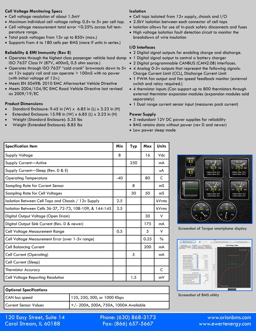
144 128

145 129

146 130

147 131

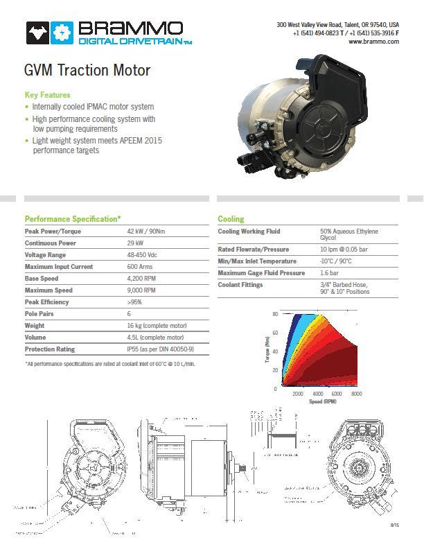
148 132

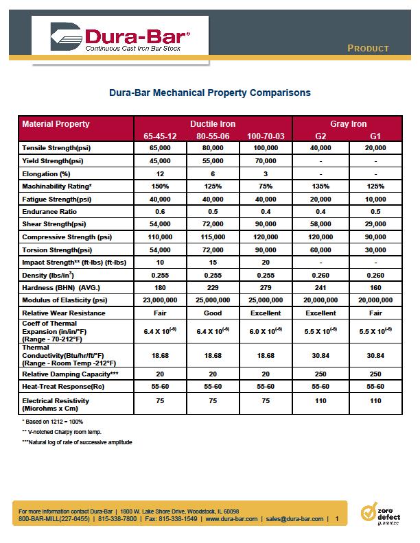
149 133

150 Appendix E Parameter Plots Appendix E encompasses battery parameter surfaces and final reduced models. Figure E.1 Open-loop voltage, Em, versus SOC and Current for 22 C. Figure E.2 Open-loop voltage, Em, versus SOC and Current for 30 C. 134

151 Figure E.3 Open-loop voltage, Em, versus SOC and Current for 40 C. Figure E.4 Series resistance, R0, versus SOC and Current for 22 C. 135

152 Figure E.5 Series resistance, R0, versus SOC and Current for 30 C. Figure E.6 Series resistance, R0, versus SOC and Current for 40 C. 136

153 Figure E.7 RC1 resistance, R1, versus SOC and Current for 22 C. Figure E.8 RC1 resistance, R1,versus SOC and Current for 30 C. 137

154 Figure E.9 RC1 resistance, R1,versus SOC and Current for 40 C. Figure E.10 RC2 resistance, R2,versus SOC and Current for 22 C. 138

155 Figure E.11 RC2 resistance, R2,versus SOC and Current for 30 C. Figure E.12 RC2 resistance, R2,versus SOC and Current for 40 C. 139

156 Figure E.13 RC1 time constant, τ1,versus SOC and Current for 22 C. Figure E.14 RC1 time constant, τ1,versus SOC and Current for 30 C. 140

157 Figure E.15 RC1 time constant, τ1,versus SOC and Current for 40 C. Figure E.16 RC2 time constant, τ2,versus SOC and Current for 22 C. 141

158 Figure E.17 RC2 time constant, τ2,versus SOC and Current for 30 C. Figure E.18 RC2 time constant, τ2,versus SOC and Current for 40 C. 142