Quantification of the Effects of Heavy Agricultural Vehicle Loading on Pavement Performance ANDREA AZARY

Transcription

1 Quantification of the Effects of Heavy Agricultural Vehicle Loading on Pavement Performance A THESIS SUBMITTED TO THE FACULTY OF THE GRADUATE SCHOOL OF THE UNIVERSITY OF MINNESOTA BY ANDREA AZARY IN PARTIAL FULFILLMENT OF THE REQUIREMENTS FOR THE DEGREE OF MASTER OF SCIENCE Lev Khazanovich, Advisor Mihai Marasteanu, Advisor March 2012

2 Andrea Azary 2012

3 Acknowledgements I can t say thank you enough to those who have paved the way to my graduation and completion of this project: To Dr. Lev Khazanovich, I couldn t have asked for a better advisor. It is from your guidance, knowledge and advice that I have expanded my interest in the pavement industry and found success with this project. Your love of pavements inspired me to attend graduate school and I am so grateful for that. To Dr. Mihai Marasteanu, for making pavement classes interesting and opening my eyes to an industry I would have never thought I would end up in. Your advice and guidance is greatly appreciated and has not gone unnoticed. To Dr. Sue Mantell, you are someone I look up to and admire. Your work ethic and passion for engineering is inspiring. I am lucky to call you a friend. To Jason Lim, when I started this project with you, I knew we would be colleagues but I didn t expect we would end up being such good friends. You helped me so much and made the transition a smooth one. Thank you for being so organized and for your hard work on this project. You made my job easy. To Dr. Shongtao Dai and MnDOT, for your guidance and assistance on this project, I can t thank you enough. This has been a tremendous opportunity to work on a project such as this and I am thankful for being given the chance to work with you. To Halil Ceylan, Simon Wang, the Iowa DOT, the Illinois DOT, the WisDOT, the Minnesota Local Road Research Board (LRRB), and the industry partners who were a part of this project, thank you so much for your involvement and for your help with this project. This was definitely a team effort and I am lucky to have worked with everyone involved. To Ki Hoon Moon, Mary Vancura, and Kyle Hoegh thank you for sharing my love of pavements and helping out at MnRoad, and helping with Construction Materials. To Mike Rief and those at WSB & Associates, for your patience as I finished this project. I have learned more about pavements in the last few months then I ever thought I would and I am grateful for the opportunity I have been given to work with you. It is an honor to be a part of your team and I am excited for the road ahead. To my family and friends, I couldn t ask for a better support system. You have been there to make me laugh and at times, to laugh at me, and I am so thankful to have you all in my life. Your constant encouragement has led me to where I am today. i

4 Abstract Started in 2007, the Pooled Fund Study, which was sponsored by the Minnesota Department of Transportation, Iowa Department of Transportation, Illinois Department of Transportation, and the Minnesota Local Road Research Board began at the MnROAD testing facility in Monticello, Minnesota. There were both flexible and rigid pavement sections implemented with strain gauges, LVDTs and earth pressure cells at the MnROAD testing facility. The objective of this study was to investigate the effects of farm equipment on the structural responses (stresses and strains) of flexible and rigid pavements. The goal of the project was to not only quantify the pavement damage caused by this heavy farm equipment compared to the damage caused by a 5-axle, 80 kip semi-truck, but to also implement and develop a computer based model that could be used to predict pavement damage. The study findings revealed that traffic wander, seasonal effects, pavement structural characteristics, and vehicle type/configuration have a pronounced effect on pavement responses to farm implements. The experimental data clearly demonstrated that all farm implements tested induced higher subgrade stresses than a standard 5-axle, 80 kip semi-truck. To minimize damage in flexible pavements due to farm implement loading, the following recommendations may be considered: increasing the number of axles while ensuring even load distribution among axles; avoiding unfavorable environmental conditions such as fully saturated and/or thawed base/subgrade or high AC temperature; and constructing a paved shoulder. ii

5 Table of Contents Acknowledgements... i Abstract... ii Table of Tables... vi Table of Figures... ix Chapter 1: Introduction Background Objectives and Methodology Organization 4 Chapter 2: Past Studies Test Sections Field Testing Testing Overview TONN Subgrade Permanent Deformation Models Base Shear Failure Criteria Fatigue Cracking Models Base Deformations Inputs Structural Responses (University of Minnesota and Iowa State University, 2010).. 26 Damage Analysis Chapter 3: Data Collection and Data Processing iii

6 3.1 Tekscan Chapter 4: Preliminary Findings Effect of Vehicle Traffic Wander Early Fall versus Late Fall Effect of Seasonal Changes Effect of Time of Testing Effect of Pavement Structure Effect of Vehicle Weight Effect of Number of Axles Effect of Axle Weight Tekscan Chapter 5: Computer Modeling (HAVED2011) Running HAVED Validation and Calibration ANALYSIS Relative Subgrade Damage Effect of Vehicle Weight Transferring Product Analysis Summary Chapter 6: Conclusions Bibliography Appendix A: Vehicle Axle Weight and Dimension Appendix B: Plots from November 2010 Testing iv

7 Appendix C: Tekscan Tire Footprints Appendix D: Pavement Response Data Fall Spring Fall Spring Fall Appendix E: Tekscan (Increased Representative Area Analysis) Appendix F: HAVED2011 Users Guide Appendix G: Projected Stress Procedure v

8 Table of Tables Table 2.1: Pavement geometric structure of flexible pavement sections... 7 Table 2.2: Pavement geometric structure of rigid pavement sections... 8 Table 2.3: List of vehicles tested Table 2.4: Overview of previous test Table 2.5: Seasonal Moduli Adjustment Factors for Base and Subgrade Table 3.1: Tekscan Analysis Summary for Vehicle T8, Axle 6, Fully Loaded Table 4.1: Number of passes at the flexible pavement section made by the Mn80 truck each season Table 4.2: Axle weights of vehicles T6, T7, and T8 at 100% in fall Table 5.1: Tekscan analysis for T7, Axle 5, 100% Loaded Table 5.2: Measured Weight of the Heaviest Axle for Each Vehicle Tested in Spring 2009 at 80% Loading Table 5.3: Testing Season, Load Level and Vehicle Axle Weight for R Table 5.4: Linear Regression Equation and Projected Weight at 100% Loading for R Table 5.5: Vehicle Axle Weights at 100% Loading Table 5.6: Maximum Measured Subgrade Stress (84PG4) Spring Table 5.7: Determination of Mn80 Subgrade Stress Factors Spring Table 5.8: Adjusted Subgrade Stresses for R Table 5.9: Linear Regression Equation for Projected Stress at 100% Loading for R Table 5.10: Projected Subgrade Stresses for Remaining Vehicles Table 5.10: SR Indexes for the Early Spring Season, 80% Loading Table 5.11: SR Indexes for the Early Spring Season, 100% Loading Table 5.12: DDI indexes for the Early Spring Season, 80% loading Table 5.13: DDI indexes for the Early Spring Season, 100% loading vi

9 Table 5.14: SR and DDI indexes for the Early Spring Season, 80% Loading, 2.5-in AC Layer Thickness, For Cell Table 5.15: Relative Rutting Damage Parameters for vehicles tested Table 5.17: Relative AC Damage Parameters for vehicles tested Table 5.18: SR Parameters for vehicles tested Table 5.19: Maximum amount of product to be carried in each vehicle Table 5.20: Measured weights at different load levels for S Table 5.21: Number of passes to haul 1,000,000 gallons of product each year for 20 years Table 5.22: Number of Axles Affected by Weight in Tank Table 5.23: DAM AC and DAM RUT Data for Cell 83 and Cell 84, 100% Loading, Fall Testing Season Table 5.24: MnPAVE Equivalent Number of ESALs Table 5.25: Equivalent Number of Passes Table A.1: Vehicle axle weights for spring 2008 test Table A.2: Vehicle axle weights for fall 2008 test Table A.3: Vehicle axle weights for spring 2009 test Table A.4: Vehicle axle weights for fall 2009 test Table A.5: Vehicle axle weights for spring 2010 test Table A.6: Vehicle axle weights for fall 2010 test Table A.7: Vehicle axle weights for fall (November) 2010 test Table E.1: Tekscan analysis for vehicle T7, Axle 5, Fully Loaded Table G.1: Maximum Measured Subgrade Stress (84PG4) Fall Table G.2: Maximum Measured Subgrade Stress (84PG4) Spring Table G.3: Maximum Measured Subgrade Stress (84PG4) Fall Table G.4: Maximum Measured Subgrade Stress (84PG4) Spring Table G.5: Maximum Measured Subgrade Stress (84PG4) Fall Table G.6: Determination of Mn80 Subgrade Stress Factors Fall vii

10 Table G.7: Determination of Mn80 Subgrade Stress Factors Spring Table G.8: Determination of Mn80 Subgrade Stress Factors Fall Table G.9: Determination of Mn80 Subgrade Stress Factors Spring Table G.10: Determination of Mn80 Subgrade Stress Factors Fall Table G.11: Adjusted Subgrade Stresses for S Table G.12: Adjusted Subgrade Stresses for S Table G.13: Adjusted Subgrade Stresses for R Table G.14: Adjusted Subgrade Stresses for T Table G.15: Adjusted Subgrade Stresses for T Table G.16: Adjusted Subgrade Stresses for T Table G.17: Adjusted Subgrade Stresses for T Table G.18: Adjusted Subgrade Stresses for T Table G.19: Adjusted Subgrade Stresses for R Table G.20: Adjusted Subgrade Stresses for G viii

11 Table of Figures Figure 2.1: Aerial view of flexible pavement test sections Cell 83 and 84 at the farm loop (Lim, 2010)... 6 Figure 2.2: Cross-sectional view of (a) thin flexible pavement section, Cell 83 (b) thick flexible pavement section, Cell 84 (Lim, 2010)... 7 Figure 2.3: Sensor layout for flexible pavement sections (a) Cell 83 (b) Cell Figure 2.4: Flexible pavement sections sensor designations for westbound lanes of (a) Cell 83 (b) Cell Figure 2.5: Example of strain response waveform Figure 2.6: Image of tested vehicles Figure 2.7: MnPAVE Mohr-Coulomb Criterion Input Screen Figure 2.8: Tekscan Tire Footprint and Equal Area Circle Representation Figure 2.9 Location of evaluation points in the structural model Figure 2.11: Plan View of Loads on Pavement Surface Figure 3.1: Tekscan hardware components (a) 5400N sensor mats (b) Evolution Handle Figure 3.2: 5400NQ sensor map layout (adopted from Tekscan User Manual (Tekscan, Inc., 2007) Figure 3.3: Outline of gross area tire footprint for axle 6 of the vehicle T8, fully loaded Figure 3.4: Determination of the x-coordinate for axle 6 of vehicle T8, fully loaded Figure 3.5: Determination of the y-coordinate for axle 6 of vehicle T8, fully loaded Figure 3.6: Example of footprint (a) measured using Tekscan (b) multi-circular area representation Figure 3.7: Example of increasing tire footprint with increasing load level Figure 4.1: Subgrade stress responses for T6 and Mn Figure 4.2: Subgrade stress versus modulus value analysis from MnLayer Figure 4.4: Subgrade stress generated by the Mn80 vehicle at Cell Figure 4.5: Longitudinal asphalt strain generated by the Mn80 vehicle at Cell Figure 4.6: Transverse asphalt strain generated by the Mn80 vehicle at Cell Figure 4.7: Failure at Cell 83 in Spring ix

12 Figure 4.8: Longitudinal strain at Cell 84 for the vehicle T6 at 100% loading in Novemebr Figure 4.9: Longitudinal strain at Cell 84 for the vehicle Mn80 in November Figure 4.10: Transverse strain at Cell 84 for the vehicle T6 at 100% loading in November Figure 4.11: Transverse strain at Cell 84 for the vehicle Mn80 in November Figure 4.12: Subgrade stress at Cell 84 for the vehicle T6 at 100% loading in November Figure 4.13: Subgrade stress at Cell 84 for the vehicle Mn80 in November Figure 4.14: Subgrade stress at Cell 84 for the vehicles tested at 100% loading in Fall Figure 4.15: Subgrade stress at Cell 84 from all vehicles tested in Fall 2009 at varying load levels Figure 4.16: Subgrade stress at Cell 84 from Mn80, T6, T7 and T8 in Fall 2009, 100% load level Figure 4.17: Subgrade stress at Cell 83 from Mn80, T6, T7 and T8 in Fall 2009, 100% load level Figure 4.18: Unadjusted AC longitudinal strain for T6 in various seasons Figure 4.19: Unadjusted AC transverse strain for T6 in various seasons Figure 4.20: Unadjusted subgrade stress for T6 in various seasons Figure 4.21: Adjusted AC longitudinal strain for T6 in various seasons Figure 4.22: Adjusted AC transverse strain for T6 in various seasons Figure 4.23: Adjusted subgrade stress for T6 in various seasons Figure 4.24: Adjusted subgrade stress for T6 for Cell 83 and Cell Figure 5.1: Second axle footprint of vehicle T7 (a) measured using Tekscan (b) multi-circular area representation Figure 5.2: Relative Subgrade Damage From the Heaviest Axle in the Spring 2009 Testing Season at 80% Loading Figure 5.3: Measured Maximum Subgrade Stresses Normalized to Mn80 Subgrade Stress Figure 5.4: Measured Subgrade Stress at 80% Loading in the Spring 2009 Testing Season Figure 5.5: Adjusted R4 Subgrade Stress vs Axle Weight Figure 5.6: Subgrade Stresses at 100% Loading Figure 5.7: Measured and Calculated Subgrade Stresses from the Vehicle S x

13 Figure 5.8: Subgrade Stress (83PG4), 100% Loading, Fall 2009 Testing Season for Mn80, T6, T7 and T8 80 Figure 5.9: AC Strain, 100% Loading, Fall 2009 Testing Season Figure 5.10: AC Strain, 100% Loading, Fall 2009 Testing Season Figure 5.11: AC Cracking Damage for Vehicles Tested, Cell 84, 80% Loading Figure 5.12: DAM RUT with Changing Asphalt Thickness Figure 5.13: DAM AC with Changing Asphalt Thickness Figure 5.14: SR with Changing Asphalt Thickness Figure 5.15: Relative Rutting Damage from Heaviest Axle; Cell 84,100% Loading Figure 5.16: Relative Rutting Damage from Heaviest Axle; Cell 83,100% Loading Figure 5.17: Subgrade Stress (84PG4) for Vehicles Mn80, T6, T7 and T Figure 5.18: Vehicle Weights and Axle Weights at 100% Loading for Fall Figure 5.19: Linear Regression for S Figure 5.20: MnPAVE analysis set up Figure 5.21: 7 TONN Road, Asphalt Damage Figure 5.22: 7 TONN Road, Subgrade Damage Figure 5.23: 10 TONN Road, Asphalt Damage Figure 5.24: 10 TONN Road, Subgrade Damage Figure A.1: Dimensions for vehicles S4, S5, and G Figure A.2: Dimensions for vehicles R4, R5, and R Figure A.3: Dimensions for vehicles T6, T7, and T Figure A.4: Dimensions for vehicles Mn80 and Mn Figure B.1: Cell 84 longitudinal asphalt strain at 100% load level in Nov 2010 for vehicles Mn80 and T Figure B.2: Cell 84 transverse asphalt strain at 100% load level in Nov 2010 for vehicles Mn80 and T6 119 Figure B.3: Cell 84 subgrade stress at 100% load level in Nov 2010 for vehicles Mn80 and T xi

14 Figure D.1: Cell 83 angled asphalt strain at 80% load level in fall 2008 for vehicles Mn80, R4, T6, and T Figure D.2: Cell 83 subgrade stress at 80% load level in fall 2008 for vehicles Mn80, R4, T6, and T Figure D.3: Cell 84 longitudinal asphalt strain at 80% load level in fall 2008 for vehicles Mn80, R4, T6, and T Figure D.4: Cell 84 transverse asphalt strain at 80% load level in fall 2008 for vehicles Mn80, R4, T6, and T Figure D.5: Cell 84 subgrade stress at 80% load level in fall 2008 for vehicles Mn80, R4, T6, and T Figure D.6: Cell 83 angled asphalt strain at 80% load level in spring 2009 for vehicles Mn80, S4, S5, R4, and R Figure D.7: Cell 83 angled asphalt strain at 80% load level in spring 2009 for vehicles Mn80, T6, T7, and T Figure D.8: Cell 83 subgrade stress at 80% load level in spring 2009 for vehicles Mn80, S4, S5, R4, and R Figure D.9: Cell 83 subgrade stress at 80% load level in spring 2009 for vehicles Mn80, T6, T7, and T8 145 Figure D.10: Cell 84 longitudinal asphalt strain at 80% load level in spring 2009 for vehicles Mn80, S4, S5, R4, and R Figure D.11: Cell 84 longitudinal asphalt strain at 80% load level in spring 2009 for vehicles Mn80, T6, T7, and T Figure D.12: Cell 84 transverse asphalt strain at 80% load level in spring 2009 for vehicles Mn80, S4, S5, R4, and R Figure D.13: Cell 84 transverse asphalt strain at 80% load level in spring 2009 for vehicles Mn80, T6, T7, and T Figure D.14: Cell 84 subgrade stress at 80% load level in spring 2009 for vehicles Mn80, S4, S5, R4, and R Figure D.15: Cell 84 subgrade stress at 80% load level in spring 2009 for vehicles Mn80, T6, T7, and T Figure D.16: Cell 83 angled asphalt strain at 100% load level in fall 2009 for vehicles Mn80, Mn102, and R Figure D.17: Cell 83 angled asphalt strain at 100% load level in fall 2009 for vehicles Mn80, T6, T7, and T xii

15 Figure D.18: Cell 83 subgrade stress at 100% load level in fall 2009 for vehicles Mn80, Mn102, and R5 150 Figure D.19: Cell 83 subgrade stress at 100% load level in fall 2009 for vehicles Mn80, T6, T7, and T Figure D.20: Cell 84 longitudinal asphalt strain at 100% load level in fall 2009 for vehicles Mn80, Mn102, and R Figure D.21: Cell 84 longitudinal asphalt strain at 100% load level in fall 2009 for vehicles Mn80, T6, T7, and T Figure D.22: Cell 84 transverse asphalt strain at 100% load level in fall 2009 for vehicles Mn80, Mn102, and R Figure D.23: Cell 84 transverse asphalt strain at 100% load level in fall 2009 for vehicles Mn80, T6, T7, and T Figure D.24: Cell 84 subgrade stress at 100% load level in fall 2009 for vehicles Mn80, Mn102, and R5 153 Figure D.25: Cell 84 subgrade stress at 100% load level in fall 2009 for vehicles Mn80, T6, T7, and T Figure D.26: Cell 84 longitudinal asphalt strain at 100% load level in spring 2010 for vehicles Mn80, Mn102, R6, and T Figure D.27: Cell 84 transverse asphalt strain at 100% load level in spring 2010 for vehicles Mn80, Mn102, R6, and T Figure D.28: Cell 84 subgrade stress at 100% load level in spring 2010 for vehicles Mn80, Mn102, R6, and T Figure D.29: Cell 84 longitudinal asphalt strain at 100% load level in fall 2010 for vehicles Mn80, Mn102, and T Figure D.30: Cell 84 longitudinal asphalt strain at 100% load level in fall 2010 for vehicles Mn80, Mn102, and G Figure D.31: Cell 84 transverse asphalt strain at 100% load level in fall 2010 for vehicles Mn80, Mn102, and T Figure D.32: Cell 84 transverse asphalt strain at 100% load level in fall 2010 for vehicles Mn80, Mn102, and G Figure D.33: Cell 84 subgrade stress at 100% load level in fall 2010 for vehicles Mn80, Mn102, and T6 157 Figure D.34: Cell 84 subgrade stress at 100% load level in fall 2010 for vehicles Mn80, Mn102, and G1158 Figure F-1: Example of HAVED2011 execution xiii

16 Chapter 1: Introduction In past years, agricultural vehicles have been exempt from any type of load restrictions when traveling on the roads (Canadian Strategic Highway Research Program, 2000). These agricultural vehicles, being one of the main types of equipment used in one of the largest industries in the United States, travel up and down roads hauling large amounts of weight, much larger than your average vehicle. In an attempt to make the agricultural industry more efficient, many of the farm equipment manufacturers have began to make the equipment larger to facilitate the transport of more products more efficiently. While this shift to larger equipment makes transporting products easier, it has led to concerns within the pavement industry as there is reason to believe these large and heavy vehicles are causing damage to public highways and local roads. As of yet, adjustments to policy and procedures for operating these types of equipment have yet to offset the damage being done to the pavement as a result of these vehicles operating by current policy, however that doesn t mean changes aren t being made. According to the 2011 Minnesota Statute , No vehicle or combination of vehicles equipped with pneumatic tires shall be operated upon the highways of this state where the total gross weight on any group of two or more consecutive axles of any vehicle or combination of vehicles exceeds that given in the following axle weight limits table for the distance between the centers of the first and last axles of any group of two or more consecutive axles under consideration. Unless otherwise noted, the distance between axles must be measured longitudinally to the nearest even foot, and when the measurement is a fraction of exactly one-half foot the next largest whole number in feet shall be used, except that when the distance between axles is more than three feet four inches and less than three feet six inches the distance of four feet shall be used (Office of the Revisor of Statutes, State of Minnesota, 2011). This is an improvement over previous laws in which the only weight restiction was to not exceed the 500 lbs per inch of tire width. While statutes like this exist, they are very difficult to enforce and are often not consistent amongst states which can make it hard for people operating farm equipment to know the laws that are in place. Research is still being done to try and find a solution to reduce the damage done to pavement by these heavy vehicle weights. 1

17 1.1 Background Due to the rising interest in this area, the South Dakota Department of Transportation performed a study in 2001 to look at the effect of various types of heavy agricultural vehicles on both flexible and rigid pavements. The study found that loaded Terragators and loaded grain carts were more damaging than a standard 18,000-lb single axle truck and recommended that these types of vehicles only be allowed to operate empty on flexible pavements and unpaved roads. This study also demonstrated the seasonal effect of pavement damage by showing that the spring season which has a wet base and subgrade is the most critical condition for rutting damage (Sebaaly, 2002). Another field study was conducted by the Iowa Department of Transportation in 1999 to look at the effect of various types of heavy agricultural vehicles on both flexible and rigid pavements. The study found that, during the spring season, because of the larger track-pavement contact area, the load associated with the tracked wagon required to induce the same stress in the ACC and PCC pavements was significantly higher than that of a 20,000-pound single-axle dual-tire semi. The limited field test and analytical results demonstrated a similar response of the two newly constructed PCC and ACC pavements under a tracked wagon. These vehicles induced lower stress and strain values in both types of pavements when compared to other loads (Fanous). The state of Iowa passed legislation which placed restrictions on the allowable loads of agricultural vehicles as a result of this study. As a follow up to the Iowa State study and the South Dakota study, the Minnesota Department of Transportation performed a study in 2001 to look at the impact agricultural vehicles had on low volume roads. The goal of their study was to try and demonstrate whether or not these vehicles were to blame for the pavement damage taking place across the state. What they found was pavement damage as a result of heavy loading but from where remained a question. Since the study was set up to include other types of heavy vehicles other than farm equipment, it was unclear as to whether the pavement damage was due to solely the agricultural vehicles or a combination of both vehicle types. At the conclusion of this study, enough questions still remained that it was suggested that a thorough field study should be conducted at the MnROAD testing facility (Phares, 2005). Started in 2007, the Effects of Implements of Husbandry (Farm Equipment) on Pavement Performance is part of the Pooled Fund study, which was started as a collaborative effort between the Minnesota Department of Transportation, the Iowa Department of Transportation, the Illinois Department of 2

18 Transportation, and the Minnesota Local Road Research Board (LRRB). This project has also had industry partners including John Deere, Husky Farm Equipment, Minnesota Custom Manure Applicators Association, Michelin Tire, Professional Dairy Producers of Wisconsin, and the Professional Nutrient Applicators Association of Wisconsin (PNAAW). 1.2 Objectives and Methodology The objective of this project was to study the effects of farm equipment on the structural responses (stresses and strains) of both flexible and rigid pavements. The responses of the farm equipment tested was compared to a standard 5-axle, 80 kip semi-truck. The study took into account the effect of axle loads, vehicle weight, vehicle speed, wheel type, and traffic wander on both flexible and rigid pavements. The MnROAD testing facility was used to construct a full-scale accelerated pavement test with resources obtained in the Transportation Pooled Fund Program. The study consisted of the construction of two flexible pavement sections and the use of two existing rigid pavement sections. The flexible pavement sections were designed as follows. The first section was designed to be a typical 10-ton road with a 5.5-inch asphalt layer and a 9.0-inch gravel base layer. The other loop was designed to be a typical 7-ton road with a 3.5-inch asphalt layer and an 8.0-inch gravel base. The two rigid pavement layers were existing concrete sections. The first was doweled and had a 7.5-inch concrete layer with a 12-inch class-6 base. The second was an undoweled section with a 5-inch thick concrete layer with a 1-inch class-1f base on top of a 6-inch class-1c subbase. In order to measure the critical responses, the flexible pavement sections were heavily instrumented with strain gauges, LVDTs, which are linear variable differential transducers, and earth pressure cells. The rigid pavement sections were instrumented with strain gauges and LVDTs. In order to capture the seasonal effects of the critical responses, testing was to be conducted in the spring and fall testing seasons. This study would also incorporate the effect of vehicle traffic wander by using video recording devices and recording the vehicle wheel path. The video records the vehicle as they travel on top of scales placed on the pavement surface. Tekscan software was also used to study the tire footprints. The tire footprints could be used to look at the effect of radial tires verses flotation tires. The objectives of this study were to compare the critical vehicle responses with respect to various variables including: vehicle load levels, vehicle speed, tire pressure, and vehicle traffic wander. This document will briefly detail the preliminary data analysis and results of the early portion of this study, 3

19 which was completed by Jason Lim at the University of Minnesota. Mr. Lim s thesis titled The Effects of Heavy Agricultural Vehicle Loading on Pavement Performance covered the test set up, data collection and preliminary data analysis portion of this study. It is the intent of this thesis to focus on the data verification and computer modeling portion of this study. To do so, this thesis will detail the damage modeling that was done to try and predict the pavement damage associated with types of farm equipment. This document only pertains to flexible pavements as the rigid pavement analysis was completed by Iowa State University as part of the Pooled Fund Study. 1.3 Organization This document contains five main chapters. Chapter 2 describes details of the pavement test set up and the procedures that were in place to run this study at the MnROAD testing facility. Chapter 3 will describe the data processing that was done in the early portion of the analysis. Chapter 4 will document the results of the study based on actual data collected. Chapter 5 includes a summary of the computer modeling that was used including the program HAVED2011 which was developed as part of this study. Chapter 6 summarizes the findings of this study and gives recommendations for helping to offset the pavement damage based on the results obtained in this project. 4

20 Chapter 2: Past Studies This project, which was started in 2007, involved extensive planning and preparation of the test sections at the MnROAD testing facility. The first stage of the study was to perform extensive field testing from which conclusions could later be drawn from. The majority of the test set up and data collection was done by Jason Lim and is detailed in his thesis, The Effects of Heavy Agricultural Vehicle Loading on Pavement Performance (Lim, 2010). The following section aims to summarize his test set up including the characteristics of the test sections that were constructed as part of this project. A study was also conducted on the TONN2010 computer application. This program was later adopted and used in the computer modeling and data validation portion of this study to run the pavement damage analysis model. This section will give a brief overview of the testing sections that were set up as well as the TONN2010 program. 2.1 Test Sections The test sections were constructed at the beginning of this study at the MnROAD testing facility. Based on the test description from the Effects of Heavy Agricultural Vehicle Loading on Pavement Performance by Jason Lim who contributed efforts to the early phases of this study, the test sections are briefly described below. As part of this study, two existing rigid test cells at the MnROAD, Cell 32 and Cell 54 were used to represent a thin layer and a thick layer, respectively. These two testing sections were used by Iowa State University to find the critical responses of concrete sections. These results will not be presented in this document. The two flexible pavement sections that were constructed were Cell 83 and Cell 84, which represent a thin section and a thick section, respectively. Figure 2.1 and Figure 2.2 below will show the aerial view and the cross sectional details of the test setup. Table 2.1 will summarize the pavement structure of the flexible pavement section. Figure 2.3 shows the rigid pavement sections at the low volume loop and Table 2.2 details the pavement structures. 5

21 Figure 2.1: Aerial view of flexible pavement test sections Cell 83 and 84 at the farm loop (Lim, 2010) (a) 6

22 (b) Figure 2.2: Cross-sectional view of (a) thin flexible pavement section, Cell 83 (b) thick flexible pavement section, Cell 84 (Lim, 2010) Table 2.1: Pavement geometric structure of flexible pavement sections Section Cell 84 (Thick section) Cell 83 (Thin section) Surface 5.5 in. thick HMA with PG in. thick HMA with PG58-34 Base 9 in. gravel aggregate 8 in. gravel aggregate Subgrade A-6 subgrade soil (existing subgrade soil) A-6 subgrade soil (existing subgrade soil) Shoulder 6 ft paved shoulder 6 ft aggregate shoulder 7

23 Traffic Direction Center Line Pavement Edge to 6 ft Aggregate Shoulder Longitudinal Offset [ft] Table 2.2: Pavement geometric structure of rigid pavement sections Section Cell 54 (Thick section) Cell 32 (Thin section) Surface 7.5 in. thick PCC 15 ft 12 ft with 1 in. dowel 5 in. thick PCC 10 ft 12 ft undoweled Base 12 in. Class-6 1 in. Class-1f 6 in. Class-1c Subgrade A-6 subgrade soil (existing subgrade soil) A-6 subgrade soil (existing subgrade soil) 20 Strain Gauge Earth Pressure Cell LVDT Thermocouple TDR Inner Wheelpath Outer Wheelpath Transverse Offset [ft] (a) 8

24 Traffic Direction Center Line Pavement Edge to 6 ft Paved Shoulder Longitudinal Offset [ft] 20 Strain Gauge Earth Pressure Cell LVDT Thermocouple TDR Inner Wheelpath Outer Wheelpath Transverse Offset [ft] (b) Figure 2.3: Sensor layout for flexible pavement sections (a) Cell 83 (b) Cell 84 In Figure 2.3 it is shown that there are three sets of strain gauge arrays that spans each lane. This was done so that the critical responses would be captured no matter what type of axle configuration the heavy agricultural equipment contained. In some cases, this led to multiple strain readings per pass as some passes hit multiple strain arrays. The outer wheel path strain array, which was installed one foot from the pavement edge, was taken to be the prime source for measurement readings. The remaining two strain gauge arrays were installed two feet apart transverse to the direction of traffic. The three earth pressure cells were then installed in line with each of the strain gauge arrays. As seen in Figure 2.4, each strain gauge set had three orientations: longitudinally, angled at 45, and transversely to the direction of traffic (Lim, 2010). There was a two-foot spacing between each strain gauge in the longitudinal direction as well as the transverse direction. The LVDTs had a three foot spacing from the pavement edge followed by a two-foot longitudinal spacing placed between each of the LVDTs. The thermocouple and TDR were installed at the center lane with a four foot spacing between them in the longitudinal direction. 9

25 (a) (b) Figure 2.4: Flexible pavement sections sensor designations for westbound lanes of (a) Cell 83 (b) Cell 84 Having multiple types of equipment is great in that it allows a diverse range of data to be collected from each vehicle pass. The only issue with this is that it is a lot of data to keep track of. This is why a detailed labeling system was developed by Jason Lim in order to keep track of this data. The first step was to keep track of the strain gauges in the strain gauge array. These were denoted as LE, AE and TE to represent the longitudinal, angled, and transverse directions, respectively. The earth pressure cells were denoted as PG (Lim, 2010). Each sensor set corresponds to the transverse offset from the pavement edge therefore numeric labels were used to denote these sensor sets. The westbound lane sensor sets were numbered 4, 5, and 6 with set 4 being closest to the pavement edge and set 6 being closest to center lane. On the eastbound lane, sensor sets were numbered 1, 2, and 3 with 1 being closest to the pavement edge and 3 being closest to center lane. Final designation for those sensors had 10

26 Strain [10-6 ] the following form: [Cell #]-[Sensor type]-[set #] (Lim, 2010). For example, the angled strain gauge farthest from the pavement edge of Cell 84 was designated as 84AE6. The LVDTs were denoted as AL1, AH2, and AV3, respectively. The LVDTs measured the displacements in the base layer in three directions: two horizontally in longitudinal and transverse directions and one vertically (Lim, 2010). Since there was only one transverse offset used for the LVDTs, the numbering scheme used for the strain gauges does not apply. For example, the horizontal LVDT in the longitudinal direction for Cell 84 was denoted as 84AL1. Figure 2.4 shows the layout of the earth pressure cells, strain gauge arrays and LVDTs with the labeling scheme detailed above. Each vehicle pass provided close to 20,000 data points per sensor including a response waveform of the asphalt strains, base deflections and subgrade stresses. Figure 2. shows an example of the strain response waveform obtained from a particular strain gauge. In order to collect all this data for each vehicle pass, some data acquisition systems were used. These systems collect response measurements at the rate of 1,200 data points per second (1,200 Hz) and each vehicle pass typically have a collection time of fifteen to eighteen seconds (Lim, 2010). The strain gauge and earth pressure cell data was collected by the Megadec-TCS system and the NI system was used to capture the LVDT data. Strain Gauge Time [sec] Figure 2.5: Example of strain response waveform 11

27 2.3 Field Testing As part of this study, the seasonal affects of the pavement responses were to be looked at. This required a well planned out testing program to be created so that available vehicles could be tested at certain times to capture as close to a fall season and spring season as possible. Due to temperature and moisture variations in spring and fall seasons, the pavement damage is usually different between the seasons. To try and capture this effect, testing was conducted twice a year in March and August. The tests conducted in August were considered to be the fall testing season even though in some instances, August can be one of the hottest months in Minnesota. However, due to constraints of equipment availability, this was often the only option available as farmers didn t have time to spare their equipment during other months. Tests conducted in March were representative of spring conditions in which the frozen layers within the pavement begin to thaw at this stage leaving the layers trapped with water. This saturation creates a cohesionless condition mainly in the base and subgrade layers resulting in a generally weakened state of the pavement structure. An additional testing season of November 2010 was also looked at to try and capture the effect of testing in early fall versus late fall. Each test provided a wealth of information including stress, strain and deflection measurements. In addition to pavement responses, specific information regarding the vehicles tested was also obtained including the vehicle axle configurations, wheel dimensions and wheel weights at varying load levels. The video recording device allowed for the traffic wander to be recorded and analyzed. The Tekscan device which was implemented in this study, allowed for the contact pressure and contact area of each tire footprint to be studied. Field testing was conducted in the spring and fall seasons of 2008, 2009, 2010 and an additional early fall testing season in A total of 14 vehicles were tested throughout the duration of this study. The two five-axle semi trucks, Mn80 (80 kip) and Mn102 (102 kip), respectively, were used as reference vehicles in this study. In addition to these semi-trucks, twelve agricultural vehicles were tested. Due to the large amounts of vehicles being studied, each vehicle was given a unique vehicle ID number to help keep track of the vehicles. An image of each of the vehicles tested as presented in Mr. Simon Wang s thesis titled, The Effects of Implements of Husbandry Farm Equipment on Rigid Pavement Performance, 12

28 is provided in Figure 2.6 (Wang, 2010). Due to the complexity of the testing schedule, a detailed summary of which vehicles were tested during which seasons is provided in Table

29 Table 2.3: List of vehicles tested 14

30 Figure 2.6: Image of tested vehicles 15

31 The test program that was implemented was done to include a range of vehicle load levels (weights), target speeds, traffic wander, and tire pressure. The test schedule was designed to include some redundancy in the vehicles tested so that a more complete and repeatable set of data could be obtained. Vehicles were tested at varying load levels including 0%, 25%, 50%, 80%, and 100%. This was done by filling the manure tanks with water and the grain cart with actual grains. MnROAD provided portable weighing scales so that the weights of each vehicle on every axle of the tested vehicles could be measured (Lim, 2010). Appendix A contains the vehicle axle weights and dimensions from the vehicles used in this study. Vehicles were also tested at various speeds including: creep, 5 mph, 10 mph, and high speed. In this study, high speed was reached at 15 to 25 mph. Due to the lack of distance at the end of the test sections for the vehicles to slow down, the vehicles were not able to be tested at operating speeds. To measure the vehicles offsets, the edges of the pavements were marked as the fog lines and the vehicles were aligned as best as they could be with target offsets of 0 in., 12 in., or 24 in. from the fog line. The actual wheel paths were determined by using the video recording devices and reading off the actual traffic wander from scales, which had been painted onto the pavement surfaces in the fall of These scales wore off in the duration of this study and were replaced with permanent steel scales. 2.4 Testing Overview Since a majority of the testing was done by Jason Lim, a summary of the testing done was taken from his thesis titled, The Effects of Implements of Husbandry (Farm Equipment) on Pavement Performance, and is included below. An additional testing season, November 2010, is included and was not part of Mr. Lim s testing schedule. The following experiments were conducted during each round of testing: Spring 2008 (March 17 th to 19 th and 24 th to 26 th ) o Tested seven vehicles; S3, S4, S5, T1, T2, T6, and Mn80. o Load levels: 0%, 25%, 50%, and 80%. o Vehicle speeds: creep, 5 mph, and 10 mph. o Vehicle offsets: 0 and 12 in. o Tire pressure for vehicle T1: 33 and 42 psi. o No measurements of traffic wander. 16

32 Fall 2008 (August 26 th to 29 th ) o Tested five vehicles; R4, T6, T7, T8, and Mn80. o Load levels: 0%, 25%, 50%, and 80%. o Vehicle speeds: creep, 5 mph, and 10 mph. o Vehicle offsets: 0 and 12 in. o Excluded need to change tire pressure. All vehicles have tire pressures which they normally operate by. o Scales were painted onto the pavement surface and videos of vehicle wheel path were recorded to estimate traffic wander. Spring 2009 (March 16 th to 20 th ) o Tested nine vehicles; S4, S5, R4, R5, T6, T7, T8, Mn80, and Mn102. o Load levels: 0%, 25%, 50%, and 80%. o Vehicle speeds: 5 mph, 10 mph, and high speed (15 to 25 mph). Excluded creep speed. o Vehicle offsets: 0 and 12 in. o Permanent steel scales were installed onto the pavement to assist in traffic wander estimation. o Failure occurred at Cell 83 westbound during test at 50% load level. Failure was propagated at 80% load level. o Failed section was patched for upcoming tests. Fall 2009 (August 24 th to 28 th ) o Tested six vehicles; R5, T6, T7, T8, Mn80, and Mn102. o Load levels: 0%, 50%, and 100%. Excluded 25% load level. o Vehicle speeds: 5 mph, 10 mph, and high speed. o Vehicle offsets: 0, 12, and 24 in. 24 in offsets were included due to recommendations from the technical committee. o Failure at patched section of Cell 83 westbound during test at 0% load level on the first day. Testing was switched to Cell 83 eastbound. o Failure at Cell 83 eastbound during test at 50% load level on the second day. Testing was switched back to Cell 83 westbound with steel sheets placed over failure section. o Failure propagated at Cell 83 westbound during test at 100% load level. 17

33 o Failure sections on both east and westbound lanes of Cell 83 were not fixed for consecutive tests. Instead, steel sheets which were placed will remain for future tests. Additional steel sheets were placed at propagated failure sections. Spring 2010 (March 15 th to 18 th ) o Tested four vehicles; R6, T6, Mn80, and Mn102. o Load levels: 0%, 50%, and 100%. o Vehicle speeds: 10 mph and high speed. 5 mph vehicle speeds were excluded. o Vehicle offsets: 0, 12, and 24 in. o Existing failure on Cell 83 westbound continued to propagate. o Both westbound and eastbound lanes of Cell 83 were dismissed from future tests. Early Fall, 2010 (August 18 th to 19 th ) o Tested four vehicles; T6, G1, Mn80, and Mn102. o Load levels: 100%. o Vehicle speeds: 10mph only. Other vehicles speeds were excluded from the test. o Vehicles offsets: 0, 12, and 24 in. Late Fall, November 2010 (November 18 th ) o Tested two vehicles; T6 and Mn80. o Load levels: 0% and 100%. Other load levels were excluded due to availability of vehicle G1. o Vehicle speeds: 10mph only. Other vehicles speeds were excluded from the test. o Vehicles offsets: 0, 12, and 24 in. 18

34 Table 2.4 summarizes the number of vehicle passes made on the flexible (AC sections) and rigid (PCC sections) pavement sections for each round of testing. Table 2.4: Overview of previous test Test Season Test Dates Vehicle Passes AC PCC Spring 2008 March 17 th 19 th & 24 th 26 th Fall 2008 August 26 th 29 th Spring 2009 March 16 th 20 th Fall 2009 August 24 th 28 th Spring 2010 March 15 th 18 th Early Fall 2010 August 18 th 19 th Late Fall 2010 November 18 th Total 3,746 1, TONN 2010 The computer program TONN 2010 was closely studied as it demonstrated the ability to perform a similar analysis to what would be needed to run pavement damage analysis models to predict the heavy agricultural vehicle damage. The TONN2010 program evaluates the damage from standard 18-kip heavy axle loads on performance of flexible pavements. The model pulls from the MnPAVE subgrade rutting damage model, the MnPAVE base shear failure model, the MnPAVE AC fatigue cracking model, and the base deformation model. In this study, the damage models from TONN2010 were adopted and used to create the program HAVED2011 which is specifically designed to evaluate the effect of heavy 19

35 agricultural equipment s performance. A brief summary of the models TONN2010 uses is provided below as well as a brief overview of how the program works. Subgrade Permanent Deformation Models The MnPAVE model, shown in Equation 2.1, for measuring permanent deformation is similar to the model presented by the Asphalt Institute (Abdulshafi, 1983). The permanent deformation being looked at is often referred to as rutting of the pavement. Rutting occurs when a poor consolidation or a lateral shift in the material layers due to repeated vehicle loads causes failure of the pavement. The MnPAVE subgrade permanent deformation model only considers rutting damage in the subgrade layer, ignoring the effects in the granular base layer c N (2.1) d Base Shear Failure Criteria Pavements can also see failure in the aggregate base. MnPAVE implements a maximum allowable stress criterion to protect this type of failure from occurring. The model MnPAVE uses is shown in Equation 2.2 and is based on the traditional Mohr-Coulomb failure criterion. 1 1critical tan 2 3 (45 ) 2 C tan(45 ) 2 2 (2.2) = internal friction angle ( ) C = cohesion 1 = maximum allowable major principal stress 3 = minor principal stress or confining pressure for the triaxial test The ratio of the stress parameters, SR= 1 critical / 1, is an indicator of how likely the base is to shear failure when the pavement is acted on by an axle load. In this ratio, 1 is the maximum shear stress and 1 critical is the critical stress value. The higher the SR value is, the less likely the base is to fail. 20

36 It is important to point out that while there is lower cohesion in the early spring due to the base layer thawing, the MnPAVE model assumes the same Mohr-Coulomb parameters, C and, for the materials regardless of the testing season. To address this limitation, TONN2010 adopted the following seasonal cohesion values C i sc i C Where Ci seasonal cohesion for the base layer for season i C = MnPAVE Late Spring default cohesion for Class 5 base (= 6 psi) sc seasonal cohesion adjustment factors; by default are equal to 10, 0.2, 1, 1.3, and 1 for i the MnPave Winter, Early Spring, Late Spring, Summer, and Fall seasons, respectively. 21

37 Figure 2.7: MnPAVE Mohr-Coulomb Criterion Input Screen Fatigue Cracking Models Another damage type faced by most asphalt concrete pavements is fatigue cracking. Typically, fatigue cracking starts at the bottom of the asphalt layer and continues to grow as is reaches the top of the asphalt layer. Tensile stresses and strains at the bottom of the asphalt layer can develop when a load is passed over the pavement and can cause the fatigue cracking to start. The severity of the stresses and strains that develop are dependent on the geometry and magnitude of the axle loading as well as the characteristics of the pavement structure. Pavement damage in fatigue cracking is typically defined as the ratio of the number of load applications to the allowable number of load applications. The Asphalt Institute lays out fatigue transfer functions which relate how many load repetitions it takes to reach varying degrees of fatigue cracking to the maximum strains at the bottom of the AC layer. This relationship is shown in Equation 2.3 (Finn et al. 1977, Chadbourn et al 2002) F1 h E N f C K (2.3) where C is a correction factor based on air voids and binder content and K F1 is a shift factor that accounts for calibration with existing R-value designs, bottom of the AC layer, and E is the AC modulus. Base Deformations h is the maximum tensile horizontal strain at the The MnPAVE rutting model does not consider rutting in the base layer. The MEPDG program uses the following equation to predict rutting in the unbound base: n o p ( soil ) s 1 ks 1 vhsoil e (2.4) r where: p(soil) = Permanent or plastic deformation in the layer/sublayer, in. n = Number of axle load applications. o = Intercept determined from laboratory repeated load permanent deformation tests, in/in. 22

38 r = Resilient strain imposed in laboratory test to obtain material properties ε o, β, and, in/in. v = Average vertical resilient or elastic strain in the layer/sublayer and calculated by the structural response model, in/in. h Soil = Thickness of the unbound layer/sublayer, in. k s1 = Global calibration coefficients; k s1 =1.673 for granular materials and 1.35 for finegrained materials. β s1 = Local calibration constant for the rutting in the unbound layers; the local calibration constant was set to 1.0 for the global calibration effort. Log W c (2.5) 10 9 C o (2.6) b1 a1m r C o Ln b9 (2.7) a9m r W c = Water content, percent. M r = Resilient modulus of the unbound layer or sublayer, psi. a 1,9 = Regression constants; a 1 =0.15 and a 9 =20.0. b 1,9 = Regression constants; b 1 =0.0 and b 9 =0.0. The field-calibrated MEPDG procedure divides the base layer into thin sublayers and computes permanent deformations in the individual sublayers (University of Minnesota and Iowa State University, 2010). In order to account for traffic wander, the vertical strains should be found at various locations. A simplified version of the MEPDG procedure was used in this study due to the complexity of the 23

39 MEPDG procedure. This simplified version is based on the observation that if the properties of the base layer do not vary with depth, then rutting in the base layer according to the MEPDG can be expressed (University of Minnesota and Iowa State University, 2010): Rut n i 1 n h (2.8) i i 1 i i Where Rut is the rutting in the base layer, i is the vertical strain in the sublayer I, and is the coefficient. If the number of sublayers is increasing then Equation 8 can be re-written as follows: Rut n n i 1 i i h h lim h dz w w (2.9) 0 0 Where w 0 is the vertical deflection at the top of the base layer, w h is the vertical deflection at the bottom of the base. Equation 2.9 suggests that limiting the difference between the vertical deflections at the top and bottom base surfaces would reduce a potential of the base rutting (University of Minnesota and Iowa State University, 2010). Inputs The inputs to the TONN2010 program included the axle load geometry and magnitude, the pavement structure characteristics and climate conditions. These were needed to compare damage caused by heavy agricultural equipment with the damage caused by a standard 18-kip single axle load. Detailed requirements for each of the group of inputs are provided below. Axle loading Tekscan measurements were used to determine the magnitude of the axle load, tire-pavement contact stresses, and the geometries of the tire footprints of the various types of heavy equipment. This was needed to characterize the effect of the axle loading on the pavement responses. It should be noted that shear contact stresses were not considered in this study and Tekscan was only capable of measuring normal stresses. Two loading problems are considered in each analysis: A half axle of a standard 18-kip single axle load A half axle of the farm equipment axle 24

40 The standard half-axle was modeled by two 3.8-in radius circular loads with pressure of 100 psi (Lim, 2010). The farm equipment half-axle loading was modeled using multiple circular loads with various radii as found using the Tekscan software. The number of the circles, their radii, and coordinates of the centroids were determined based on the results of Tekscan measurements. Figure 2.8 presents the tire footprint from Tekscan and the corresponding representation of the footprint by a series of circular loads. The applied pressure was summed to be the same for each circle and was determined by dividing the load magnitude by the footprint area (Lim, 2010). Figure 2.8: Tekscan Tire Footprint and Equal Area Circle Representation Pavement Structure The pavement matrix can greatly affect the structural responses (stresses, strains, and deflections) due to axle loading. To accurately determine pavement damage, the characteristics of a pavement structure need to be considered. As inputs, the user needs to provide information such as pavement layer thicknesses and elastic properties of the layers. In this study, a simple pavement matrix was considered consisting of an asphalt layer, a base layer, a subgrade layer and a stiff bedrock layer. The base layer was assumed to be 12-in thick, so it may also include an upper portion of the compacted subgrade (Lim, 2010). The subgrade depth to the bedrock may vary from 12 to 240 inches. A subgrade depth to the bedrock represents a condition where no bedrock is present. 25

41 For each layer, in the pavement system, except the bedrock, the user should provide elastic properties (moduli of elasticity and Poisson s ratios) as well as the interface conditions. In this study, it was assumed that all layers are fully bonded, which is a typical assumption in flexible pavement analysis. The following Poisson s ratios were assumed (University of Minnesota and Iowa State University, 2010): Asphalt layer: 0.35 Base: 0.4 Subgrade: 0.45 Climatic Inputs Climatic effects were looked at as part of this study but were also involved in evaluating pavement damage. Obviously, in warmer seasons, the pavement structure becomes less stiff and can influence the amount of damage present. In this study, MnPave was used. MnPAVE considers five seasons (Ovik, 1999): Early Spring: The season when the aggregate base is thawed and nearly saturated, but the subgrade remains frozen. Late Spring: The season when the aggregate base has drained and regained partial strength, but the subgrade is thawed, near saturated, and weak. Summer: The season when the aggregate base is almost fully recovered, but the subgrade has only regained partial strength. Fall: The season when both the aggregate base and subgrade have fully recovered. Winter: The season when all pavement layers are frozen. Table 2.5: Seasonal Moduli Adjustment Factors for Base and Subgrade Layer Winter Early Late Summer Fall Spring Spring Base Subgrade Structural Responses (University of Minnesota and Iowa State University, 2010) 26

42 The following Structural Response explanation was taken from the task report titled Damage Analysis Model, which was part of this study. To compare damage caused by heavy agricultural equipment and the standard axle loading, the critical pavement responses (strains and deflections) are computed using the layered elastic program MnLAYER (Khazanovich, 2007) for each season. The subsequent damage analysis requires determination of the following structural responses: Maximum vertical strain at the top of the subgrade Maximum difference of vertical deflections at the top and bottom surfaces of the base Minimum ratio of the critical stress and first principal stress at the base mid-depth Maximum horizontal strain at the bottom of the AC layer It should be noted that the vertical displacements at the bottom of the asphalt layer are equal to the vertical displacements at the top of the base layer. The vertical displacements at the bottom of the base layer are equal to the vertical displacements at the top of the subgrade. These observations permit significant reduction in the number of points at which the responses have to be determined. Since simple footprint geometry is assumed for the standard single axle load, the most likely locations of the maximum responses can be narrowed down based on the past experience. Therefore, the responses are determined for the following locations: Point A. Bottom of the AC layer, under the center of the wheel Point B. 6-inches into the base layer, under the center of the wheel Point C. Top of the subgrade layer, under the center of the wheel Point D. Top of the base layer, mid-distance between the wheels Point E. 6-inches into the base layer, mid-distance between the wheels Point F. 12-inches below the top of the base layer, mid-distance between the wheels 27

43 A B C D E F Figure 2.9 Location of evaluation points in the structural model The maximum principal horizontal strain computed at point A is used in the subsequent AC damage calculation. The vertical strain computed at point C is needed for subgrade rutting damage analysis. Stresses computed at points B and E are used to compute the principle and critical stresses as defined by Equation 2.1. These stresses are used to compute the strength to stress ratios. The lowest strength to stress ratio, SR c, is used in the subsequent analysis as defined in Equation Geometry of the agricultural equipment tire footprint can be quite complex. Therefore, it is difficult to guess locations of the maximum responses prior to the analysis. To address this challenge, the responses were evaluated for the following layers of points (see Figure 2.10): Layer A. Bottom of the AC layer Layer B. Mid-depth of the base layer Layer C. Top of the subgrade layer Each layer consisted of 100 points organized in either a 10 X 10 or a 5 X 20 mesh equally spaced in x- and y- directions (see Figure 2.15). The horizontal coordinates of the points did not vary from layer to layer. The coordinates of the end points is either a user-provided input or determined from the minimum and maximum horizontal coordinates of the centers of the circular loads in the agricultural equipment tire footprint. 28

44 From horizontal strains computed at each point of Layer A, the maximum horizontal strain is determined and used in the subsequent AC damage calculation. The maximum vertical strain among the vertical strains computed for points in Layer C is needed for subgrade rutting damage analysis. Critical and principal stresses computed at points of Layer B are used to compute the strength to stress ratios. The lowest strength to stress ratio, SR c, from all the loads being considered, is used in the subsequent damage analysis. Finally, the maximum difference between deflections of the points in Layer A and the corresponding points in Layer C is used in the base damage analysis. Figure 2.10: Location of evaluation points in the structural model 29

45 Figure 2.11: Plan View of Loads on Pavement Surface The structural responses should be computed for each MnPAVE season. Although the layer thicknesses, load geometry and locations of the evaluation points do not vary from season to season, the layer moduli are adjusted to account for seasonal variations in asphalt temperature as well as subgrade and base moisture content. To determine representative seasonal AC moduli values, the average seasonal pavement temperature need to be calculated. TONN2010 adopted the MnPAVE procedure. The following equation is used: 1 34 Tpi Tai 1 6 (2.10) z 4 z 4 Where T pi = average seasonal pavement temperature at depth z for season i ( o F) T ai = average seasonal air temperature for season i ( o F) z = depth at which material temperature is to be predicted, in The average seasonal air temperature for any Minnesota location can be found from the MnPAVE design software climate screen. 30

46 After the seasonal pavement temperatures are determined, the corresponding AC moduli are determined using the equation developed by Lukanen et al, (1998) from the analysis of the Long Term Pavement Performance (LTPP) Seasonal Monitoring Program (SMP) data: slope T seas T ref E seas E ref 10 (2.11) The magnitude of the slope in the equation above depends on the individual characteristics of the mix such as the binder properties and aggregate characteristics. The range encountered in the LTPP SMP study for the slope was roughly bounded by to In this study, a slope value of was adopted. The elastic properties of unbound materials are moisture dependent. Since moisture conditions vary from season to season, the backcalculated base and subgrade moduli are adjusted using the following equations: bsi E base, i Ebase * b day (2.12) ssi E subgr, i Esubgr* s day (2.13) where E base = backcalculated base modulus E base,i = average base modulus for season i bs i = base modulus season adjustment factor for season i. b day = base modulus adjustment factor accounting for a difference in the moisture conditions for the test day. By default it is equal to the season adjustment factor for the season of testing. E subgr = backcalculated subgrade modulus E subgr,i = average subgrade modulus for season i 31

47 ss i = subgrade modulus season adjustment factor for season i. s day = subgrade modulus adjustment factor accounting for a difference in the moisture conditions for the test day. By default it is equal to the season adjustment factor for the season of testing. Damage Analysis For this study, a new program, HAVED2011 was created from the basic methodology behind the TONN2010 program to be able to quantify the damage done by the various heavy agricultural vehicles in comparison to the standard 18-kip vehicle. After the critical responses are determined for each season, the damage analysis is performed to calculate relative damage and damage indexes. It involves a subgrade rutting damage analysis, a base shear failure analysis, an AC fatigue cracking damage analysis and a base deformation analysis. The following equations are taken from the Damage Analysis Model (University of Minnesota and Iowa State University, 2010). The allowable number of load repetitions is determined using the following equation: 2.35 vi NRUT, i (2.14) N, = allowable number of ESALs for season i in terms of subgrade damage. RUT i B,i = maximum vertical subgrade strain for season i combinations of elastic properties To determine a relative damage in terms of rutting for season i from a passage of a heavy axle of an agricultural equipment, the following equation can be used: (2.15) Similarly, the number load applications to failure in AC cracking was determined in HAVED2011 using the following equation: 32 (2.16)

48 Where A,i = maximum principal horizontal strain at the bottom of AC layer for season i combinations of elastic properties E ACi = AC elastic modulus for season i. To determine a relative damage in terms of AC cracking for season i from a passage of a heavy axle of an agricultural vehicle, the following equation can be used: (2.17) HAVED2011 uses the ratios of the first principle stress and critical stress and the difference in the base deflections to evaluate bearing capacity of the pavement and obtain a road rating based on the maximum axle load rather than the number of load applications. In this study, the TONN2010 approach was modified for estimation of the maximum allowable axle loading. The following indexes were suggested: SR i 1 critical 1 (2.18) DDI i 1 DW i (2.19) Where 1 = major principal stress 1 critical = critical stress defined by equation (2) DDI = differential deflection index DW i = difference in the vertical deflections of the top and bottom base surfaces (in microns) computed for a season i. The following failure criteria are suggested: 33

49 * SR i SR (2.20) * DDIi DDI i (2.21) * SR and * DDI i are the calibration parameters depending on pavement material properties The procedure described above is incorporated into a FORTRAN code (University of Minnesota and Iowa State University, 2010). The program incorporates MnLAYER for simulation of pavement loading by an 18-kip single axle load and the axle of interest. After that, it computes the relative damage in subgrade rutting and AC cracking induced by the axle of interest compared to the standard 18-kip axle, as well as the maximum SR and DDI parameters. 34

50 Chapter 3: Data Collection and Data Processing As part of this study, tire footprints and traffic wander data needed to be collected and processed. This section details the Tekscan software that was used to measure the tire footprints as well as the procedure used to collect the traffic wander data. The majority of this data collection was done by Jason Lim and is discussed in this thesis, The Effects of Heavy Agricultural Vehicle Loading on Pavement Performance. The procedure used for collecting the pavement response data will be reviewed in this document. Further analysis and validation was performed on the Tekscan measurements since Mr. Lim completed the data collection and preliminary data analysis portion of this study. This analysis and validation will be discussed in the following sections. Data validation was done by looking at measurements from different vehicles or testing seasons than were presented in Mr. Lim s thesis. 3.1 Tekscan As described above as part of the inputs for using the TONN2010 program, the Tekscan software was implemented in this study. The Tekscan measurements were used to obtain the relative pressure distributions for each wheel of the equipment being studied at various load levels. Tekscan uses four sensorial mats (model 5400 N) and four data handles (Evolution Handles) with attached USB cables to measure the tire footprints and the vertical contact pressure of the vehicles used in this study. This equipment is shown in Figure 3.1. A picture of the Tekscan set up is shown in Figure 3.2. (a) (b) Figure 3.1: Tekscan hardware components (a) 5400N sensor mats (b) Evolution Handle 35

51 Sensorial mat A Sensorial mat B Sensorial mat C Sensorial mat D Figure 3.2: 5400NQ sensor map layout (adopted from Tekscan User Manual (Tekscan, Inc., 2007) As the vehicles traversed the mats, the data was collected using the I-Scan version 5.90 software. As described in the Tekscan users guide, the Tekscan set up and testing involved the following steps (Tekscan, Inc., 2007). 1. The 5400N sensorial mats and Evolution Handles were placed as shown in Figure 3.2. Sensorial mats were placed on top of a flat steel sheet to protect it from the underlying rough pavement surface. These mats were also protected with plastic sheets to prevent damage from the vehicle pass. 2. Handles A and B are positioned from left to right along the top of the array while handles C and D are positioned from left to right along the bottom of the array. 3. Sensorial mats A and D were placed with the words This Side Up facing right side up while sensorial mats B and C were positioned with the words This Side Up facing down. 4. All sensorial mats were clamped to the corresponding handles according to their positions. 36

52 5. The handles were connected to a computer and checks were performed to ensure that all connections were secured and complete. 6. The Sensor OK LED must be lit green to indicate that sensorial mats were correctly inserted to the handles. The Power LED must be lit green to indicate handles are receiving power and has been initialized by the computer. 7. The I-Scan version 5.90 software was launched and the 5400NQ sensor map was selected together with all four available handles. 8. Sensitivity of sensorial mats and recording parameters were configured prior to conducting the test. Note that equilibration of the sensors was not performed during actual testing due to lack of resources (uniform pressure loading apparatus). 9. Test vehicles were driven over the sensorial mats of the 5400NQ setup while the I-Scan software records information from the pass. Note that the 5400NQ setup was wide enough to only accommodate one side of the vehicle s axle. 10. As the vehicle proceeds over the sensorial mats, the vehicle operator was not allowed to execute any steering adjustments, accelerate, or decelerate while the tires are on or approaching the mats. The purpose for using the Tekscan software was to capture the tire footprint of the vehicles as well as the applied tire pressure. In the agricultural industry, it is known that a larger tire footprint and a lower inflation pressure is ideal due to the fact that is helps reduce rutting and compaction of the soil in the field. This was one of the parameters this study wanted to look into. A comparison was done specifically between the effect of pavement damage with radial tires versus the damage done with flotation tires. The relative pressure distributions obtained using the Tekscan mats were then adjusted using the total wheel weight and the actual pressure distribution was obtained. This procedure is summarized below. 1. The measurements obtained in each vehicle pass were first saved into a.fsx file format. 2. Using I-Scan software, the previously saved.fsx file was opened. 3. The frame containing the clearest image of a complete tire footprint was selected. 4. A linear calibration was performed using the Tools pull-down menu and entering in the appropriate length, force and pressure units. 5. The Frame button was selected and the number of the frame selected in step 3 was entered. 37

53 6. The total applied force which corresponded to the wheel load at the tested load level was entered. 7. The calibration file was saved in a.cal format, separate from the movie which was previously saved in a.fsx format. These steps were done for each wheel per half axle. There was then a process to estimate the tire s contact area along with its load distribution from the Tekscan measurements. This process is detailed below. 1. The previously saved.fsx file was opened using the I-Scan software. The associated.cal file which corresponds to the wheel being considered is then selected. 2. The Save ASCII tab was selected from the File menu. A Save ASCII pop-up window appeared. Under Data Type, Frame Data was selected and under Movie Range, Current Frame was selected. 3. This file was then saved in an.asf file format. 4. This.asf file could then be opened using Microsoft Excel. Each individual sensel of the Tekscan sensorial mat corresponds to an individual cell in the Excel spreadsheet. Most of the cells show a value of 0 meaning no pressure was exerted onto that sensel of the Tekscan mat. The nonzero values represent the pressure that was exerted onto that sensel on the mat. Each sensel on the Tekscan mat has dimensions of.6693 in X.6693 in. This makes the area of a sensel, in In order to easily identify sensels and corresponding cells in Excel, a coordinate system was introduced. The origin was said to be the bottom left hand corner cell in which a value of 0 was present. Coordinates for each cell in both the horizontal and vertical direction were then available. 6. Zooming in and out of the Excel spreadsheet allowed the outline of the gross area of the tire footprint to be identified by highlighting all the non-zero values. This is shown in Figure 3.3 for axle 6 of the vehicle T8 fully loaded. 38

54 Figure 3.3: Outline of gross area tire footprint for axle 6 of the vehicle T8, fully loaded 39

55 7. A check on the contact area and contact pressure found directly through the I-Scan software was then performed. This was done by multiplying the number of non-zero cells by the sensel area of in 2 to obtain the net contact area, A net. Dividing the known wheel load by this value gave the contact pressure. 8. The overall gross area of the tire footprint was then broken down into roughly an equal number of horizontal and vertical cells to form square-like boxes representative of the net area. It needed to be ensured that no squares overlapped. The dark borders in Figure 3.3 outline the representative areas. It can be seen that the tire footprint for axle 6 of vehicle T8 fully loaded, was broken down into six representative areas. 9. The square boxes were then represented as a circular area with an evenly distributed load in the layered elastic analysis. The squares were then transformed into a circle with equal area. 10. The centroid of each section weighted by the applied pressure of each sensel was determined. Pressure at sensel i was denoted as P i located at coordinates (x i, y i ) (Lim, 2010). 11. The x-coordinate and y-coordinate of the centroid of section n was denoted as x n and n xi Pi Pi n n respectively where; x and y n yi Pi Pi n This step is shown in Figure 3.4 and Figure 3.5 below. n y n, 40

56 Figure 3.4: Determination of the x-coordinate for axle 6 of vehicle T8, fully loaded 41

57 Figure 3.5: Determination of the y-coordinate for axle 6 of vehicle T8, fully loaded 42

58 12. The coordinates computed in the previous step had no units. Therefore, they were multiplied by the sensel dimensions of.6693 in. in both directions to convert into inches. 13. The number of non-zero cells within the section was multiplied by the sensel area of in 2 and the area of each section, A n, was found. 14. Knowing the area of each section, the radius, r n could be found. 15. The load applied, F n onto each section n was determined through F n A A n net F total, where F total is the applied wheel load. A table summarizing this information for axle 6 of vehicle T8, fully loaded is shown in Table 3.1. Table 3.1: Tekscan Analysis Summary for Vehicle T8, Axle 6, Fully Loaded T8 Axle 6 Full Analysis Total Area Centroid Centroid Wheel Load x y x(in) y(in) Average Pressure Section x y x (in) y (in) Area (in^2) Radius Load Pressure The size and location of the representative circular areas represent the load distribution of the footprint. Figure 3.6 shows an example of the estimated contact area for a footprint. Since these are representative areas, it is possible that these circular areas could overlap. Figure 3.7 shows that with increasing load level, there is increased tire pressure, as you can see from the larger tire footprint. 43

59 (a) (b) Figure 3.6: Example of footprint (a) measured using Tekscan (b) multi-circular area representation 44

60 Figure 3.7: Example of increasing tire footprint with increasing load level The tire footprints for all the vehicles tested at varying load levels is provided in Appendix C of this thesis. An updated Tekscan analysis was performed on all the vehicles in this study as part of the data validation on the data collected by Jason Lim in the early portions of this study. The procedure presented above was followed with each vehicle. Table 3.1 shows the results of a Tekscan analysis for one particular axle on one particular vehicle under one particular loading scenario. This Tekscan summary information was used as part of the input file in the modeling portion of this study. This will be discussed further in Chapter 5. 45

61 Chapter 4: Preliminary Findings Once the testing was complete, conclusions and observations could be made from the data collected. The results of the effect of traffic wander, seasonal changes, early fall versus late fall, the effect of time of testing, the effect of the pavement structure, the effect of vehicle and axle weight, the effect of vehicle type, and the effect of the number of axles were found by Jason Lim in his thesis, The Effects of Heavy Agricultural Vehicle Loading on Pavement Performance and will be summarized briefly in this chapter. Additional data validation was performed on Mr. Lim s findings. His results were verified by looking for similar trends using different vehicles or testing seasons than were presented in his thesis. 4.1 Effect of Vehicle Traffic Wander The video recording device used in this study allowed the affect of vehicle offset to be viewed. The target offsets for the vehicles to follow were set up prior to testing and the operators of the vehicles were instructed to follow that transverse offset as best they could. The actual traffic wander was then viewed from the video and the transverse distance to the vehicle as read from the steel scale was recorded. The testing showed that the effect of traffic wander was important and affected the maximum response that would be recorded with the vehicle pass. Not only did it show to impact the maximum response specific to each vehicle and pass, it also affected which axle would give the maximum response. Figure 4.1 below shows that the subgrade stress readings are greater when the vehicle passed more directly over the sensor. It be noted that the relative offset refers to the rear axle relative offset and denotes the distance from the center of the most rear wheel axle relative to the location of the sensor. It can be seen that the greater the offset in either direction, the lower the subgrade stress reading. This trend is seen amongst all vehicles. 46

62 Figure 4.1: Subgrade stress responses for T6 and Mn Early Fall versus Late Fall Figure 4.1 indicates that in both August 2010 and November 2010, the subgrade stresses generated by T6 were higher than those generated by the Mn80 vehicle. It can also be seen that the subgrade stresses for both T6 and Mn80 were higher in August 2010 than in November This is most likely due to the stiffening of the pavement due to the temperatures dropping. The stiffer the pavement matrix becomes, there will be less flexibility in the matrix leading to less damage being done to the pavement. 4.3 Effect of Seasonal Changes The effect of seasonal changes was shown in the data obtained in this study. In colder months, the base and subgrade layers begin to freeze and become stiff. When the ground begins to warm up again, the frozen layers begin to thaw out leaving a less stiff layer and often times excess moisture in the layers. 47

63 In order to try and capture a seasonal effect, field testing was conducted each year in the spring and fall seasons with an additional testing session added in November 2010 to capture the effect of early fall versus late fall which was discussed in section 4.2. The Mn80 standard 80-kip truck used by MnROAD was used as the control variable in this study. Table 4.1 shows the number of passes that were made on the flexible pavement sections each season by the Mn80 truck. Table 4.1: Number of passes at the flexible pavement section made by the Mn80 truck each season Day Number of Passes S08-day1 2 S08-day2 4 F08-day1 15 F08-day2 20 F08-day3 5 S09-day1 15 S09-day2 13 S09-day3 12 S09-day4 20 F09-day1 29 F09-day2 28 F09-day3 41 F09-day4 44 S10-day1 68 S10-day2 71 S10-day3 72 F10-day1 68 F10-day2 74 Nov10-day1 60 TOTAL 661 The vehicles tested during each season were heavily dependent on which vehicles were available as well as what vehicles the industry wanted to see tested. The testing set-up tried to ensure that each type of 48

64 vehicle was at least tested in both the fall and the spring seasons so that a direct comparison could be made based on seasonal effects eliminating the effects of simply having different vehicles tested each season. Due to availibility of vehicles, this was not always an option and in some instances, vehicles with similar configurations were substituted in the study. While the original tractor may have been substituted with similar vehicles, the tankers were always consistent throughout testing seasons and the capacity and axle configurations were kept as close to the original as possible. As temperatures increase, it is expected that the pavement thaws and the stiffnesses decrease. The decrease in stiffness is often represented by a decrease in the modulus value. An exercise was done using MnLayer to generate the subgrade stresses that would be generated as the modulus value increases. The results of this analysis are shown in Figure 4.2. The results show that an increase in the modulus decreases the subgrade stress. This is what would be expected, as a less stiff layer will feel more pressure from an applied load, which is why this plot shows higher subgrade stresses for lower modulus values. Figure 4.2: Subgrade stress versus modulus value analysis from MnLayer 49

65 Figure 4.4 through Figure 4.6 shows the subgrade stress, longitudinal asphalt strain and transverse asphalt stress from the Mn80 vehicle for each day of testing for Cell 84. These figures not only show significant seasonal variation, but also daily fluctuations due to changes in temperatures from day to day. Figure 4.4: Subgrade stress generated by the Mn80 vehicle at Cell 84 Figure 4.5: Longitudinal asphalt strain generated by the Mn80 vehicle at Cell 84 50

66 Figure 4.6: Transverse asphalt strain generated by the Mn80 vehicle at Cell 84 Figures 4.5 and 4.6 show lower measured asphalt strain values in the spring testing seasons. Higher strain values would be expected when temperatures are warmer. This is because warmer temperatures lead to a less stiff pavement matrix which leads to higher strains. The higher strain values in the fall suggest that the pavement is more susceptible to fatigue like damage in the fall than in the spring. Figure 4.4 shows that the subgrade stresses were slightly larger in the fall than in the spring. The large subgrade stress value for the first day of testing in the Spring 2009 testing season could be attributed to the variation in the freeze-thaw cycle in spring. Generally during spring, the thawing of the previously frozen base and subgrade layers occurs which reduces the strength and stiffness of those layers. The reason for this unusually high subgrade stress value could be due to a subgrade layer which was still frozen. No strong correlation between subgrade stresses and season of testing was observed. However, base or subgrade strength is usually lower in spring than in fall. 51

67 Figure 4.7: Failure at Cell 83 in Spring 2009 Figure 4.7 shows failure at Cell 83 in the Spring 2009 testing season. There was a longitudinal crack that developed along with significant rutting close to the sensors. The section was repaired in time for Fall 2009 testing. This may explain the high angled strain ratings what were obtained at Cell 83 in the Fall 2009 testing season. Despite the section being repaired, the failure most likely caused damage to the pavement structure that affected the material properties. Failure occurred again in Fall Effect of Time of Testing Not only were seasonal effects considered, but the time of day the testing occurred was also looked at. During each day of testing it generally warmed up in the afternoon. For example, during the time of testing in one day the pavement temperature varied from 80 ºF to 87 ºF in the fall of 2009 and from 40 F to 50 F in the spring of 2009 (Lim, 2010). To account for this temperature increase, test workplans included testing vehicles on a given day of testing in both the morning and afternoon under similar conditions (axle weights, speed of testing, etc) in each case. The morning was said to represent the colder temperature in the day, when the asphalt layer was still stiffer due to the cooler temperature. The afternoon was representative of a time when the sun had a change to warm up the temperature and therefore the asphalt layer leading to less stiffness in the asphalt layer. 52

68 Figure 4.8 through Figure 4.13 shows the effect of the maximum axle response measurements for the morning testing sessions versus the afternoon testing sessions for the vehicles T6 and Mn80 which were tested in the November 2010 testing season. These figures show the maximum response across the pavement width along with the relative offset of the last axle. The measured responses in the afternoon were higher than those measured in the morning. Figure 4.8: Longitudinal strain at Cell 84 for the vehicle T6 at 100% loading in Novemebr 2010 Figure 4.9: Longitudinal strain at Cell 84 for the vehicle Mn80 in November

69 Figure 4.10: Transverse strain at Cell 84 for the vehicle T6 at 100% loading in November 2010 Figure 4.11: Transverse strain at Cell 84 for the vehicle Mn80 in November

70 Figure 4.12: Subgrade stress at Cell 84 for the vehicle T6 at 100% loading in November 2010 Figure 4.13: Subgrade stress at Cell 84 for the vehicle Mn80 in November

71 Figure 4.14: Subgrade stress at Cell 84 for the vehicles tested at 100% loading in Fall 2009 Figure 4.14 shows the subgrade stress maximum responses in the morning and afternoon testing sessions for all the vehicles tested in Fall 2009 at 100% loading. Measured asphalt strains and subgrade stresses were higher in the afternoon tests when the asphalt temperature was higher for all vehicles. Most increases in visible pavement distresses were observed in the afternoon test sessions. 4.5 Effect of Pavement Structure Before failure of Cell 83, tests were being conducted on both Cell 83 and Cell 84 at the MnROAD testing facility to compare the effects of the pavement structure. As discussed in Chapter 2, Cell 84 was built as the thicker pavement section and Cell 83 was considered the thinner section due to thinner layers throughout the structure. Cell 84 was designed as a typical 10-ton road, meaning a road which can be legally traversed by an 80-kip semi truck, or in our study, the Mn80 vehicle. Cell 83 was designed as a 7- ton road, so a slightly lower capacity than Cell 84. The maximum responses for each vehicle were looked at both for Cell 83 and Cell 84. Some of the strain gauges failed so a direct comparison between strains with the same orientation was not always an option. In the event that this occurred, the larger value between the longitudinal and transverse strains from Cell 84 were compared to the angled strain from Cell 83. In all seasons tested, the results were the same as presented in these figures. The thicker the asphalt and base layers, the lower the measured strains and subgrade stresses. 56

72 Another structural feature built into this study was the effect of a paved shoulder. Cell 84 was designed to have a paved shoulder, Cell 83 had an aggregate shoulder. The presence of a paved shoulder was found to reduce damage potential. In the absence of a paved shoulder, allowing the vehicles to drive in the middle of roads (away from the edge) reduces the risk of pavement failure. 4.6 Effect of Vehicle Weight The effect of vehicle weight was looked at by testing vehicles at various load levels. There is a general trend that the longitudinal and transverse strain values increase with increasing vehicle weight. Figure 4.15 below shows the effect of increasing the load level amongst all the vehicles tested in Fall 2009 at Cell 84. It can be seen that except at a 0% load level, Mn80 has the lowest subgrade stresses out of all the vehicles tested. This trend is seen in both the spring and fall testing seasons. Figure 4.15: Subgrade stress at Cell 84 from all vehicles tested in Fall 2009 at varying load levels Additional plots from Jason Lim s thesis, showing the pavement responses generated by the tested vehicles and the Mn80 vehicle are shown in in Appendix D. 4.7 Effect of Number of Axles It was realized from looking at the gross vehicle weight that there could be an effect relating to the axle configuration of the vehicles. Depending on the number of axles, the weight could be distributed differently on different axles which could also affect the measured responses. The study showed that 57

73 pavement damage is governed by axle weight, not the gross vehicle weight, therefore, it is important to ensure even load distribution among axles. The design of agricultural vehicles has been changing to legally meet the axle weight restrictions in place on public roads. This can be accomplished by adding axles to the vehicles to help distribute the weight. The T6, T7 and T8 vehicles that were available in this study were used to look at this effect since these vehicles had similar configurations except the T6 vehicle had 4 axles, the T7 vehicle had 5 axles and the T8 vehicle had 6 axles. The T6 vehicle had a capacity of 6,000 gallons. The T7 vehicle had a capacity of 7,300 gallons. The T8 vehicle had a capacity of 9,500 gallons. Table 4.2 shows the axle weights of the T6, T7, and T8 vehicles that were loaded at 100% in Fall 2009 to compare the effect of the number of axles. Table 4.2: Axle weights of vehicles T6, T7, and T8 at 100% in fall 2009 Equipment Axle T6 (6,000 gal) T7 (7,300 gal) T8 (9,500 gal) [lb] [lb] [lb] Tractor Axle 1 8,100 6,900 14,800 Axle 2 21,400 19,800 25,200 Axle 3 26,500 26,300 23,300 Tanker Axle 4 33,500 26,200 23,700 Axle 5 26,000 23,500 Axle 6 23,700 Total vehicle weight 89, , ,200 Table 4.2 shows that although T6 has the lowest total vehicle weight, the last axle, Axle 4, of the T6 vehicle has the highest distributed axle weight of 33,500 lbs. The T8 vehicle, despite having the highest gross vehicle weight, has a back axle with only 23,700 lbs on it. It is interesting to point out that the T8 vehicle s highest loaded axle was actually Axle 2, with a weight of 25,200 lbs. In this study, the first two 58

74 axles correspond to the tractor so those axle weights will generally not change significantly with increasing load levels. The remaining axles are those belonging to the tankers and will see an increase with an increase in the load level. Figure 4.27 and Figure 4.28 show the subgrade stress responses of these vehicles at 100% loading in Fall 2009 both for Cell 83 and Cell 84. Figure 4.16: Subgrade stress at Cell 84 from Mn80, T6, T7 and T8 in Fall 2009, 100% load level Figure 4.17: Subgrade stress at Cell 83 from Mn80, T6, T7 and T8 in Fall 2009, 100% load level The results from Figure 4.16 and Figure 4.17 may be a bit surprising. Despite T6 having the lowest gross vehicle weight, it shows to produce the highest subgrade stress values. The T7 and T8 vehicles are 59

75 roughly the same, although the T8 vehicle appears to be slightly lower than the T7 subgrades stress values. This showed that for tankers with a larger capacity, adding axles can potentially reduce the subgrade stresses that are generated. This trend was not seen with asphalt strains. 4.8 Effect of Axle Weight While the overall trend showed an increase in the stress and strain responses with increasing weight, there was some inconsistency with this trend that led to looking more closely at the effect of axle weight. The inconsistency was reasoned to be attributed to the increase in gross vehicle weight not being evenly distributed amongst the axles, but also due to some temperature conditions. To try and eliminate any climatic effects from influencing the data, a correction factor, d i, was introduced. Taken from (Lim, 2010), the correction factor is based on responses obtained from the control vehicle Mn80 as shown in Equation 4.1. T 6i T 6i Mn80o Mn80i d T 6i i (4.1) Where T 6i is the adjusted subgrade stress from the rear axle of vehicle T6 for ith day T 6i is the measured subgrade stress from the rear axle of vehicle T6 on ith day Mn80o is the reference subgrade stress for vehicle Mn80 Mn80i is the measured subgrade stress for vehicle Mn80 on ith day d i is the ratio between measured subgrade stress on ith day and reference stress for vehicle Mn80 This same form of the equation was used to adjust the strain values for climatic effects. In this case, strain measurements were substituted for stress measurements. The following is taken from (Lim, 2010) and explains the procedure which was used to adjust for these climatic effects. To maintain consistency the correction factor is always based on the responses generated by the heaviest axle of Mn80. The adjustment process was the performed on the maximum response generated by the heaviest axle of the vehicle of interest across the entire pavement width. This step is important to 60

76 identify the relationship between axle responses and axle weight instead of using the maximum response across the vehicle axles and total vehicle weight which may be misleading (Lim, 2010). The response measurements of the Mn80 vehicle on the fourth day of testing during the Fall 2008 testing season was selected as the reference Mn80 response. Figure 4.18 and Figure 4.19 show the unadjusted strain responses for the T6 vehicle for various testing seasons. Figure 4.20 shows the unadjusted stress responses for the T6 vehicle for various testing seasons. Figure 4.21 Figure 4.23 shows the adjusted strain and stress responses. This adjustment was done for each type of strain response for all the vehicles. The purpose of doing this was to eliminate the daily fluctuations in measured responses. Figure 4.24 shows a comparison in the adjusted subgrade stress responses for the vehicle T6 for Cell 83 and for Cell 84. Figure 4.18: Unadjusted AC longitudinal strain for T6 in various seasons 61

77 Figure 4.19: Unadjusted AC transverse strain for T6 in various seasons Figure 4.20: Unadjusted subgrade stress for T6 in various seasons 62

78 Figure 4.21: Adjusted AC longitudinal strain for T6 in various seasons Figure 4.22: Adjusted AC transverse strain for T6 in various seasons 63

79 Figure 4.23: Adjusted subgrade stress for T6 in various seasons Figure 4.24 shows a comparison in the adjusted subgrade stress responses for the vehicle T6 for Cell 83 and for Cell 84. There appears to be a linear relationship between the stress and axle weight, with this figure clearly showing that the stress increased as the axle weight increased. Figure 4.24: Adjusted subgrade stress for T6 for Cell 83 and Cell 84 64

80 4.9 Tekscan The Tekscan procedure was described in section 3.1 and was used in this study to show that the tire footprints changed not only for differing tire types but also for varying load levels. The Tekscan measurements also provided information about the loading pattern and loading distribution of the tires. This information along with the contact area and contact pressure was used in the computer modeling part of this study and will be discussed in the following chapter. 65

81 Chapter 5: Computer Modeling (HAVED2011) Part of the problem with this study was limited availability to testing equipment when it was needed. Farmers are using their equipment during the times it would be ideal to test these vehicles. Computer modeling was done in this study to not only validate the data that was obtained in the study but also to provide means for accurately predicting the pavement damage without extensive data analysis. The HAVED2011 program was developed based on the TONN2010 model which was described in this report. The damage analysis procedure developed in this study has been implemented into a FORTRAN program HAVED2011. To execute the program, the user has to create an input file containing information about the pavement structure, climatic data, layer moduli and loads. A complete User Guide for using HAVED2011 is included in Appendix F in this report. 5.1 Running HAVED2011 An input file summarizing the Tekscan analysis was created for each axle of each vehicle. The input files summarize the pressure, radius, and x and y coordinates of the equal area circle representations created in doing the Tekscan analysis. This file is also where the user can input the size of the mesh to be used in the analysis. Table 5.1 provides a sample of the information obtained from the Tekscan analysis described in Section 3.1. The example shown is for the vehicle T7. 66

82 Table 5.1: Tekscan analysis for T7, Axle 5, 100% Loaded T7Houle7300FullAxle5 Total Area Centroid Centroid Wheel Load x y x(in) y(in) Average Pressure Section x y x (in) y (in) Area (in^2) Radius Load Pressure Table 5.1 shows the resulting data obtained from doing a multi-circular breakdown of the tire footprint instead of using one loaded circular area. The pressure, radius and x-coordinate and y-coordinate are used to run the HAVED2011 program and predict damage for each vehicle. An example of what is meant by a multi-circular breakdown is shown in Figure

83 (a) (b) Figure 5.1: Second axle footprint of vehicle T7 (a) measured using Tekscan (b) multi-circular area representation An analysis was run in which a tire footprint was broken into much smaller multi-circular representations. This was done to see the effect creating a smaller mesh would have on running the HAVED2011 model. The example Tekscan data shown here had the T7, Axle 5, tire footprint broken into 12 representative circular areas. This analysis broke the T7, Axle 5, tire footprint into 67 representative circular areas. The results of this Tekscan analysis are provided in Appendix E. The results of running the model did not show a significant difference past breaking a tire footprint down into greater than 20 sections. Therefore, the process detailed in Section 3.1 held and is what was used in the Tekscan analysis. 5.2 Validation and Calibration The HAVED2011 program was used to run damage models to predict which vehicles caused the greatest damage. The program calculated this damage terms of a vehicles rutting damage (DAMRUT), asphalt damage (DAM AC) its stress ratio (SR) which was the ratio of the critical stress to the measured stress, and its differential deflection index (DDI) which was a measure of the pavement deflections caused by the vehicles. Maximum values of subgrade stresses and asphalt strains were extracted for each test day 68

84 of each test season. Pavement responses from the 5-axle 80-kip MnRoad semi truck (Mn80) were used to adjust responses. To validate the procedure, Spring 2009 test data at an 80% loading level for Cell 84 was simulated for each vehicle tested in that season. Table 5.2 shows the measured weight of the heaviest axle for each vehicle. Figure 5.2 shows the resulting relative subgrade damage from the heaviest axle. One can observe that according to the simulation a passage of the heaviest axle of each vehicle resulted in higher subgrade damage than from a passage of the heaviest axle of the Mn80 truck. The highest damage was predicted for vehicle R4. Table 5.2: Measured Weight of the Heaviest Axle for Each Vehicle Tested in Spring 2009 at 80% Loading Vehicle Axle Measured Weight of Heaviest Axle (lbs) R4 2 39,340 S3 2 26,960 S4 3 21,460 S5 3 20,040 T6 4 22,460 T7 3 22,840 T8 4 21,280 Mn80 4 and 5 34,080 To verify these predictions, the maximum measured subgrade stresses from each vehicle from all the measurements made on that day were determined (see Figure 5.3) and compared with the predicted relative rutting damage. One can observe that indeed all the vehicles induced higher subgrade stresses than the Mn80 truck and the Terragator R4 induced the highest stress. The relative ranking of subgrade stresses was mostly similar to the ranking of the relative subgrade damage. There was, however, one noticeable discrepancy. The measured subgrade stress from vehicle S4 was lower than from many 69

85 vehicles, like T6, T7, and T8, whereas the predicted relative rutting damage was very similar if not higher. Figure 5.2: Relative Subgrade Damage From the Heaviest Axle in the Spring 2009 Testing Season at 80% Loading *Note: Only vehicles tested in the Spring 09 testing season are included in Figure 5.2 as the comparison in Figure 5.3 uses only vehicles tested in the Spring 09 testing season. Figure 5.3: Measured Maximum Subgrade Stresses Normalized to Mn80 Subgrade Stress 70

86 To investigate this discrepancy, an additional analysis of the simulated and measured data was conducted. First, the predicted subgrade stresses were determined for each vehicle and normalized to the subgrade stresses from the Mn80 truck. The trend of the calculated subgrade stresses followed the trend of the predicted relative subgrade damage and the discrepancy between the ranking of the predicted measured and calculated stresses from S4 and other vehicles was observed. After that, a detailed comparison of the measured stresses from the S4 and T6 vehicles was conducted. Figure 5.4: Measured Subgrade Stress at 80% Loading in the Spring 2009 Testing Season Projected Stress Procedure Despite having an extensive testing schedule, not every load level for every vehicle was able to be tested. Most vehicles were tested at an 80% load level, but not every vehicle was tested at a 100% load level. The Mn80 and Mn102 trucks were always considered to be 100% loaded. In order to make not only a fair comparison amongst vehicles, but also to help validate the HAVED2011 model, a projected stress procedure was developed to predict the heaviest vehicle axle weights and stresses at 100% loading. The projected heaviest axle weights at 100% loading were found using a linear regression. For as many seasons as testing was performed in, a linear regression was made for each specific vehicles load levels tested and corresponding vehicle axle weights. This was the case with the vehicle R4, which was only 71

87 ever tested at 0, 25, 50 and 80% load levels. Table 5.3 shows the testing season, load level, and corresponding vehicle axle weights for the vehicle R4. Table 5.3: Testing Season, Load Level and Vehicle Axle Weight for R4 Testing Season Fall 2008 Spring 2009 Load Level Vehicle Axle Weights Using all the data available for each vehicle, a linear regression equation was developed from which the vehicle axle weight at 100% loading could be projected. This information is summarized in Table 5.4 below for the vehicle R4. Table 5.4: Linear Regression Equation and Projected Weight at 100% Loading for R4 Slope Intercept Projected Weight At 100% In the event that a vehicle was in fact measured at 100% loading, the heaviest vehicle axle weight measured was used in the analysis instead of using a projected heaviest axle weight at 100% loading. This was the case with the vehicle G1 for example. In Fall 2010, the G1 vehicle was measured at 100% loading and the corresponding heaviest axle weight was 57,200 lbs. This is the axle weight that was used in determining the projected stress at 100% loading. Table 5.5 summarizes the vehicle axle weights at 100% loading. 72

88 Table 5.5: Vehicle Axle Weights at 100% Loading Mn Mn R R S S T T T T T R G In order to determine the projected stress values at 100% loading, the seasonal effects had to be taken out of the measured stress values. To accomplish this, the Fall 2008 testing season was designated as the baseline season and all other testing season stress values were normalized against this season. The first step was to find the measured maximum subgrade stress values (84PG4) for the vehicles tested during each testing season. An example of this can be seen in Table 5.6. Table 5.6: Maximum Measured Subgrade Stress (84PG4) Spring 2008 Maximum Measured Subgrade Stress (84PG4) Spring 2008 Vehicle 0% 25% 50% 80% [psi] [psi] [psi] [psi] Mn NA NA S S T The remaining testing season s maximum measured subgrade stress (84PG4) data can be found in Appendix G. 73

89 The baseline was then selected as the maximum measured stress from the Mn80 vehicle in the Fall 2008 testing season at an 80% load level, which was psi. A Mn80 subgrade stress factor was developed to normalize the measured Mn80 subgrade stress values during each season to the Mn80 subgrade stress value measured during the baseline season, Fall The Mn80 subgrade stress factor was simply the ratio of the maximum measured subgrade stress value at a given load level, during a given season to that of the maximum measured subgrade stress value for the Mn80 vehicle at an 80% loading in the Fall 2008 testing season. Table 5.7 summarizes the Mn80 subgrade stress factors for the Spring 08 season at the respective load levels tested during that season for the Mn80 vehicle. The ratio calculated was specific to the day of testing. It is known that the Mn80 truck was always considered fully loaded. Table 5.7: Determination of Mn80 Subgrade Stress Factors Spring 2008 Spring 2008 Fall 2008 Load Level Test Measured Subgrade Stress (psi) (For Mn80) Measured Subgrade Stress (psi) (For Mn80) Mn80 Subgrade Stress Factor 0% % The Mn80 subgrade stress factors for the remaining seasons can be found in Appendix G. To correct the maximum measured subgrade stresses of all the vehicles in all the seasons tested, each maximum measured subgrade stress for a given season, load level and vehicle was adjusted by dividing the maximum measured subgrade stress value for that specific vehicle, season and load level by the Mn80 subgrade stress factor corresponding to the same load level and testing season. This is shown in Table 5.8 for the vehicle R4. 74

90 Table 5.8: Adjusted Subgrade Stresses for R4 Season - Load Level Maximum Measured Subgrade Stress (psi) Mn80 Subgrade Stress Factor Axle Weight (lbs) Adjusted Subgrade Stress (psi) S09-0% S09-25% S09-50% S09-80% F08-0% F08-50% F08-80% The adjusted subgrade stresses for all the remaining vehicles can be found in Appendix G. Using all the data available for the maximum axle weights as well as the adjusted subgrade stresses for each vehicle, a linear regression was then used to project the subgrade stress at 100% loading. The adjusted subgrade stress versus the axle weights was first plotted for each vehicle. This is seen in Figure 5.5 for the vehicle R4. From this, a regression equation was developed. 75

91 Figure 5.5: Adjusted R4 Subgrade Stress vs Axle Weight This information for the regression equation is summarized in Table 5.9 below for the vehicle R4. Table 5.9: Linear Regression Equation for Projected Stress at 100% Loading for R4 Slope Intercept Projected Weight At 100% Projected Stress At 100% After plugging in the projected weight at 100% loading, the projected stress at 100% loading is obtained. The remaining projected stresses are summarized below in Table

92 Table 5.10: Projected Subgrade Stresses for Remaining Vehicles Vehicle Slope Intercept Projected Weight At 100% Projected Stress At 100% S S R T T T T T R G The relative order of the subgrade stresses for the vehicles tested is shown in Figure

93 Figure 5.6: Subgrade Stresses at 100% Loading Measured responses are affected by many factors, including a relative position of the wheel path with respect to a sensor. As it can be observed from Figure 5.4, although T6 resulted in higher subgrade stresses, it is not clear if readings from S4 were not adversely affected by the wander, i.e. there was no passage directly over the pressure gage. To eliminate the effect of traffic wander on the measured maximum stresses, a procedure for the stress adjustment was developed. From the MnLAYER predictions, a stress profile was developed and matched with the measured stresses (see Figure 5.5). It can be observed that MnLAYER predicts a similar effect of the traffic wander on the subgrade stress magnitude. Moreover, it indicates that the most critical position of the axle with respect to the pressure gage sensor was not evaluated in the field test. Therefore, this phenomenon partially explains lower measured subgrade stresses for S4 than for other vehicles like T6, T7, and T8. Another factor that may contribute to the discrepancy between the measured stresses and the predicted damage is a possible error in the axle weight measurement. In Spring 2008 the axle weight of the heaviest axle of S4 was 20,240 lbs. In Spring 2009 it was 21,460 lbs. We compare this finding with the weight of another axle which did not change significantly between seasons (19,320 and 19,520 lb in 2008 and 2009, respectively). Taking these considerations into account, one can conclude that the predicted rutting damage agrees fairly well with the measured subgrade stresses. 78

94 Figure 5.7: Measured and Calculated Subgrade Stresses from the Vehicle S4 Cell 83 (3.5-in AC section) failed in Spring of Throughout the duration of the study, Cell 84 (5.5-in AC section) did not show significant distresses even after having been loaded at 100% load level in Fall 2009 and subsequent test seasons. Many factors could have caused the pavement failure so it is hard to pinpoint the exact cause of failure, however based on the data from this study and previous knowledge; educated guesses can be made as to what caused the failure. It was reasoned that the pavement first failed in the base or subgrade layer, although AC cracking could not be completely ruled out as the cause of failure. It was specifically seen that the base layer was very weak in the Spring 2009 testing season. Cell 83 also, did not have a paved shoulder and it has since been shown that the presence of a paved shoulder reduces damage potential. In the absence of a paved shoulder, allowing vehicles to drive in the middle of roads (away from the edge) reduces a risk of pavement failure. In this study, all vehicles in all seasons resulted in high subgrade stresses and were higher than the standard 18-kip vehicle. Subgrade stresses were specifically very high in the Fall 2009 testing season as can be seen in Figure

95 Figure 5.8: Subgrade Stress (83PG4), 100% Loading, Fall 2009 Testing Season for Mn80, T6, T7 and T8 The rutting damage analysis presented above gives a good indication of a relative damage caused by axle loading during a rutting damage accumulation process, but is not suitable for failure analysis. To address this limitation, two other HAVED2011 indexes were evaluated. Table 5.11 presents the stress ratios calculated for the vehicles participating in Spring 2009 testing for 80% load level and Table 5.12 presents the stress ratios for all the vehicles for 100% load level. One can observe that none of the vehicles exhibited a SR lower than 1 for Cell 84 even for the 100% load level. Meanwhile, every vehicle exhibited a SR less than 1 for Cell 83 and several vehicles exhibited a SR less than 0.9, which demonstrates higher potential for failure. 80

96 Table 5.11: SR Indexes for the Early Spring Season, 80% Loading Vehicle Cell 83 Cell 84 R S S S T T T Mn Mn T T Table 5.12: SR Indexes for the Early Spring Season, 100% Loading Vehicle Cell 83 Cell 84 R S S S T T T Mn Mn T T A similar analysis was performed for the DDI parameter. Tables 5.13 and Table 5.14 summarize the results for the vehicles in Spring 2009 testing for 80% load level and for all the vehicles for 100% load 81

97 level, respectively. One can observe that for Cell 84 this parameter is computed to be greater than 1.4 for all vehicles at 80% loading, whereas all the vehicles except the Mn80 truck and T2 vehicle resulted in this parameter lower than 1.3 for the Spring 2009 testing season. For 100 percent loading, all vehicles resulted in a DDI greater than 1.3 for Cell 84, whereas for Cell; 83 several vehicles resulted in a DDI close to or less than 1. 82

98 Table 5.13: DDI indexes for the Early Spring Season, 80% loading Vehicle Cell 83 Cell 84 R S S S T T T Mn Mn T T Table 5.14: DDI indexes for the Early Spring Season, 100% loading Vehicle Cell 83 Cell 84 R S S S T T T Mn Mn T T A forensic study conducted on the failed portion of Cell 83 indicated that the asphalt layer thickness on the failed subsection was less than designed and equal to 2.5 in. To evaluate the effect of reduced 83

99 asphalt thickness, Cell 83 was simulated with a 2.5-in thick AC layer as well. Table 5.15 presents the computed SR and DDI parameters for all the vehicles from the Spring 2009 testing season. One can observe that a decrease in AC thickness lead to further decrease in the SR and DDI parameters. Many vehicles exhibited a SR less than 0.8 and a DDI less than 0.9. This means that limiting these parameters are good indicators of failure potential and must be limited. For the materials used in construction of the MnROAD test cells, it is reasonable to assume that SR and DDI values exceeding 1 and 1.3, respectively should be considered safe. On the other hand, SR and DDI values less than 0.8 and 0.9, respectively, should be considered as indicators of high failure potential. Table 5.15: SR and DDI indexes for the Early Spring Season, 80% Loading, 2.5-in AC Layer Thickness, For Cell 83 Vehicle SR DDI R S S S T T T Mn Mn T T Data obtained in this study led to the belief that cracking in the AC layer is less likely to cause failure. This idea was formed partially by considering strain data obtained from the Peak-Pick analysis. In Spring 2009, only S4 and S5 vehicles resulted in higher strains than strains caused by the Mn80 truck. The S4 and S5 vehicles were not tested in Fall 2009 when the east-bound lane of Cell 83 failed. Mn80 and Mn102 trucks were responsible for the highest strains in the Fall 2009 testing season. 84

100 Figure 5.9: AC Strain, 100% Loading, Fall 2009 Testing Season Figure 5.10: AC Strain, 100% Loading, Fall 2009 Testing Season The relative AC damage calculated in this study (see Figure 5.11) also shows that the damage from the farm equipment was similar to or less than the damage from the Mn80 truck. It should be noted, however, that AC layer failure cannot be completely ruled out as the cause of failure. The AC strains are very sensitive to the vehicle pass. It is quite possible that the measured strains did not record the highest strains. Also, only bottom surface AC strains were measured. Longitudinal cracking is often 85

101 caused by high top surface strains. Measurement and modeling of these responses was out of the scope of this study. Figure 5.11: AC Cracking Damage for Vehicles Tested, Cell 84, 80% Loading Asphalt Thickness Sensitivity Analysis The developed model was used to perform an asphalt thickness sensitivity analysis and compare the relative damage of the vehicles with varying asphalt thicknesses. The relative rutting damage, relative AC damage, and SR parameters for vehicles tested were obtained for asphalt thicknesses of 2.5, 3.5, 4.5 and 6 inches, respectively. The results are presented in Table 5.16, Table 5.17 and Table 5.18 as well as Figure 5.12, Figure 5.13 and Figure 5.14 below. The results were consistent with what would be expected. As the thickness of the asphalt layer increased, the relative amount of damage compared to the 18-kip single axle load increased in most cases. This can be explained by reasoning that for thin pavements there is a redistribution of the loads on the pavement. When the pavement becomes thicker, the tire footprint becomes less important and the axle weight takes on greater importance. This is most likely why the relative damage becomes higher. It is important to note that when the pavement becomes thicker, it can sustain more passes of the 18-kip single axle load, i.e. the absolute damage from each axle pass is reduced. Also, as it can be observed from Table 5.16 and Figure 5.14 an increase in asphalt thickness increases the SR parameter which indicates lower potential of base failure. 86

102 Table 5.16: Relative Rutting Damage Parameters for vehicles tested DAM RUT 2.5 Inches 3.5 Inches 4.5 Inches 6 Inches R S S S T T T Mn Mn T T Figure 5.12: DAM RUT with Changing Asphalt Thickness 87

103 Table 5.17: Relative AC Damage Parameters for vehicles tested DAM AC 2.5 Inches 3.5 Inches 4.5 Inches 6 Inches R S S S T T T Mn Mn T T Figure 5.13: DAM AC with Changing Asphalt Thickness 88

104 Table 5.18: SR Parameters for vehicles tested SR 2.5 Inches 3.5 Inches 4.5 Inches 6 Inches R S S S T T T Mn Mn T T Figure 5.14: SR with Changing Asphalt Thickness 89

105 ANALYSIS Relative Subgrade Damage Not every vehicle was tested at 100% capacity. To address this limitation, maximum axle weights were projected for the vehicles tested at 80% capacity and below. The subgrade rutting analysis program was performed for both Cell 83 (3.5-in AC section) and Cell 84 (5.5-in AC section). Figure 5.15 and Figure 5.16 provide the resulting relative rutting damage from the heaviest axle at 100% loading for Cell 84 and Cell 83, respectively. One can observe that every vehicle tested in this study produces higher subgrade rutting damage than a standard Mn80 truck. Therefore, if a pavement has weight restrictions for commercial traffic it should also apply to heavy agricultural equipment. One can also observe that the R4, R6, G1, and T6 vehicles at 100% loading induce significantly higher subgrade rutting damage than the remaining vehicles. It should be noted, however, that according to the manufactures, the R4, R6, and G1 vehicles should not be loaded at 100% capacity when traveling on paved surfaces. Figure 5.15: Relative Rutting Damage from Heaviest Axle; Cell 84,100% Loading 90

106 Figure 5.16: Relative Rutting Damage from Heaviest Axle; Cell 83,100% Loading Effect of Vehicle Weight A fully loaded T6 vehicle resulted in much higher subgrade stresses than the T7 and T8 vehicles (see Figure 5.17). The relative rutting damage analysis presented above confirms this observation. In this study, the T6, 6000 gal vehicle at 100% loading weighed 60.0 kips. A T7, 7300 gal vehicle at 100% loading weighed 79.5 kips. Finally, the T8, 9500 gal vehicle weighed 94.2 kips at 100% loading as shown in Figure One can see that the relative rutting damage is not correlated to the gross vehicle weight. At the same time, the maximum axle weights measured in this study were 33.5, 26.3, and 23.7 kips for vehicles T6, T7, and T8, respectively. A significantly higher maximum axle weight explains why the T6 vehicle resulted in higher measured subgrade stresses and computed rutting damage. The results showed the importance of the load distribution along axles. This is very important especially for a two axle tanker. We found that increasing the number of axles is beneficial even though the vehicle weight increases. 91

107 Figure 5.17: Subgrade Stress (84PG4) for Vehicles Mn80, T6, T7 and T8 Figure 5.18: Vehicle Weights and Axle Weights at 100% Loading for Fall 2009 Transferring Product Analysis Vehicle comparisons were made throughout this project, and were typically compared against the standard Mn80, 6,000 gallon truck, and the Mn102, 8,500 gallon vehicles. An analysis was performed to address the question, which vehicle is the least damaging if you have 1,000,000 gallons of product that needs to be moved? This analysis was performed on both the 7-ton and 10-ton roads for design lives 92

108 of 20 years assuming the product is moved every year. The method of this analysis and the results are presented in this section. The first step to doing this analysis was to find the total weight of the material that could be carried in the tanker of each vehicle. This meant taking the weight of the vehicle filled with a product and subtracting the weight of the empty vehicle so that only the amount of product in the tank remained. Table 5.19 summarizes the maximum amount of product that could be carried in each vehicle. Table 5.19: Maximum amount of product to be carried in each vehicle Summary of Vehicle Weights Used in Analysis Vehicle Heaviest Weight Full Heaviest Weight Empty Difference R6 74,700 42,050 32,650 S4 60,409* 25,000 35,409 S5 64,590* 28,100 36,490 T6 89,500 39,710 49,790 T7 105,200 45,100 60,100 T8 134,200 58,200 76,000 T1 91,975* 44,500 47,475 T2 63,742* 30,780 32,962 The values shown with an asterisk in Table 5.19 represent values that have a projected weight at 100% loading. The vehicles S4, S5, T1, and T2 were not measured at 100% loading so these values were projected based on a linear regression of the levels that were tested and the associated vehicle weights. The projected weight at 100% loading was found based on the other measured weights found for each vehicle. An example of finding projected weight is shown for the S4 vehicle below. The projected weights for the other vehicles were found in the same manner. For the vehicle S4, the load levels tested and their measured weights at each load level were obtained and are shown in Table

109 Table 5.20: Measured weights at different load levels for S4 S4 Load Level (%) Measured Weight (lbs) 0 24, , , ,100 From these measured weights, a linear regression was performed and the projected value at 100% loading could then be found from the resulting equation from the linear regression. The graph and equation for S4 is shown in Figure Figure 5.19: Linear Regression for S4 Once these values were found, the number of passes required for each vehicle assuming a material with a specific weight other than water was being moved was found. This was done by assuming there was 1,000,000 gallons of the product to be moved, and assuming the material weighed 8.3 lbs per gallon. It was assumed that 1,000,000 gallons of the material was moved every year for a period of 20 years. Thus, the number of passes was found by the following equation: 94

110 Where the maximum amount of product is the maximum amount of product each vehicle can hold as is shown in Table This equation then gives the total number of passes it would take to haul 1,000,000 gallons of the product each year for 20 years. This data is presented in Table Table 5.21: Number of passes to haul 1,000,000 gallons of product each year for 20 years. Vehicle Number of Passes R6 5,084 S4 4,688 S5 4,549 T6 3,334 T7 2,762 T8 2,184 T1 3,497 T2 5,036 Mn80 3,333 Mn102 2,353 To get a sense of the equivalent damage moving this product will produce, it needs to be distributed amongst the appropriate number of axles being affected for each vehicle. Table 5.22 shows the number of axles the weight is considered to act on for each vehicle. 95

111 Table 5.22: Number of Axles Affected by Weight in Tank Vehicle Number of Axles R6 1 S4 2 S5 2 T6 2 T7 3 T8 4 Mn80 2 Mn102 2 T1 2 T2 2 In order to find the equivalent number of passes, the DAM AC and DAM RUT values for Cell 83 and Cell 84 at 100% loading was also needed. These values were obtained using the HAVED2011 program and are summarized in Table Table 5.23: DAM AC and DAM RUT Data for Cell 83 and Cell 84, 100% Loading, Fall Testing Season Cell 83 Cell 84 Vehicle DAM AC DAM RUT DAM AC DAM RUT R S S T T T Mn Mn T T

112 The allowable number of ESALs was also needed to find the damage from moving the product. This was found using MnPAVE. The set-up used in the MnPAVE analysis is shown below in Figure Figure 5.20: MnPAVE analysis set up The results of MnPAVE are summarized in Table Table 5.24: MnPAVE Equivalent Number of ESALs Allowable Number of ESALs 7-TONN road (3.5-in thick AC pavement ) 10-TONN road (5.5-in thick AC pavement ) AC Fatigue 1,400,000 13,400,000 Subgrade Rutting 320, ,000 The following equation demonstrates how to find the AC Fatigue damage using the DAM AC index values. This same calculation can be done using the DAM RUT index values. In order to find the equivalent number of passes, the following calculation was used. 97

113 In this equation: Number of Axles = The number of axles affected by weight in tank DAM AC = The DAM AC index values found from HAVED2011 Number of Passes = The total number of passes it would take to haul 1,000,000 gallons of the material each year for 20 years. MnPAVE Equivalent Number of ESALs = The equivalent number of ESALs as found from the MnPAVE analysis. It should be noted that T6 has two axels which are affected by the weight of the tanker, however the measured data showed significant differences in the way the weight is distributed amongst the back two axels. Because of this finding, the DAM AC and DAM RUT indexes were not simply doubled to account for two axels, but rather HAVED2011 was run for each back axle individually and the DAM AC and DAM RUT values for the back two axels were summed to obtain a more accurate result. The equivalent number of passes was found for both Cell 83 and Cell 84. The results are summarized in Table Table 5.25: Equivalent Number of Passes Cell 83 Damage Cell 84 Damage Vehicle AC Fatigue AC Fatigue AC Fatigue DAM RUT R S S T T T Mn Mn T T

114 Figure 5.21: 7 TONN Road, Asphalt Damage Figure 5.22: 7 TONN Road, Subgrade Damage 99

115 Figure 5.23: 10 TONN Road, Asphalt Damage Figure 5.24: 10 TONN Road, Subgrade Damage These results are shown in Figures above. It can be seen in looking at the results of the subgrade damage that all vehicles exhibit higher subgrade damage in equivalent passes than the Mn80 100

116 and Mn102 vehicles. It appears that as you move to the 10-ton road the asphalt damage is negligible. In the case of the 7-ton road, while the damage may appear to be negligible, it is important to remember that the results presented are for the fall testing season. The results will be higher in spring and a spring loading restriction may still be required. It is also seen that in general the asphalt damage is less than the subgrade rutting damage, meaning it is important to look at the subgrade rutting damage. It was shown that the 10-ton road will feel less damage than the 7-ton road most likely due to the thickness being greater on the 10-ton road. Summary As a result of the damage analysis model, the relative amounts of damage for the vehicles tested were modeled. It was found that increasing the number of axles was beneficial even if the vehicle weight increases. The R4, R6, and G1 vehicles were found to have higher amounts of relative damage. It should be noted, however, that according to the manufactures, the R4, R6, and G1 vehicles should not be loaded at 100% capacity when traveling on paved surfaces. It was also found as a result of this analysis that the results of the subgrade damage that all vehicles exhibit higher subgrade damage in equivalent passes than the Mn80 and Mn102 vehicles. It appears that as you move to the 10-ton road the asphalt damage is negligible. In the case of the 7-ton road, while the damage may appear to be negligible, it is important to remember that the results found were for the fall testing season. The results will be higher in spring and a spring loading restriction may still be required. An asphalt sensitivity analysis was performed and showed that the thicker your asphalt layer becomes, the more you are increasing the strength and stiffness of the pavement matrix and the less damage will be developed. Other results of the damage analysis showed that cracking in the AC layer is less likely to cause failure. In Spring 2009, only S4 and S5 vehicles resulted in higher strains than strains caused by the Mn80 truck. Mn80 and Mn102 trucks were responsible for the highest strains in the Fall 2009 testing season. In this study, all vehicles in all seasons resulted in high subgrade stresses and were higher than the standard 18-kip vehicle. 101

117 Chapter 6: Conclusions The results of this study were very informative both to people in the agriculture industry who had been looking for an extensive study on the effects of their equipment on both flexible and rigid pavements as well as to local and state transportation agencies looking for ways to improve the service lives of their pavements. The 7-ton road and 10-ton road constructed at the MnROAD facility allowed extensive testing to be done in real life settings with real life applications. This allowed the pavement responses from various types of heavy agricultural equipment to be tested looking at factors such as the impacts of number of axles, axle loads, differing tire footprints, etc. The responses from the agricultural vehicles were then compared to those from a standard 5-axle semi-truck to gauge whether the agricultural vehicles were more or less damaging. If vehicles were found to be more damaging than a standard 80- kip vehicle, then recommendations for how to combat the level of damage could be made. The effects of environmental conditions were found to be fairly significant. The base and subgrade layers were found to be affected by moisture conditions in those layers and temperature was found to affect the behavior of the asphalt and concrete layers. The extensive testing program (testing twice a year for three years) allowed for a vast amount of information to be analyzed and took into account a range of environmental conditions. Testing during the season when spring load restrictions are typically enforced allowed this study to capture the effect of heavy farm equipment loading on pavements during spring thawing conditions. The fall testing seasons provided data from a time when the ground may be more frozen, but a time that typically sees heavy traffic of heavy agricultural equipment. The computer modeling that was a part of this project was very beneficial and developed a means for predicting the pavement damage that would be generated from the types of heavy agricultural equipment that were looked at in this study. The HAVED2011 program that was developed used the experimental data results to calibrate and validate the model and improve the predictions for damage to the pavement. The key findings from this study from both the experimental data collected and the analytical modeling are summarized as follows: 102

118 The data obtained from testing at the MnROAD facility showed that the pavement structure, axle weight, traffic wander, season of testing, and the vehicle type/configuration of the vehicle impacted the pavement responses that were collected. The failure in Spring 2009 of Cell 83 which was designed as a 7-ton road demonstrated the importance of pavement thickness. The lack of a paved shoulder at this section could have contributed to the severe rutting and structural failure that was observed. The cracking was witnessed to have started in the thin AC section of Cell 83. The failure of this design showed that 7-ton roads are not sufficient to handle the type of loads seen by the types of heavy agricultural equipments that were used in this study. The fact that there was no significant damage seen in the 10-ton designed section, Cell 84, shows that this type of road does not require a spring load restriction on commercial traffic. Cell 84 was designed to have a thicker asphalt layer and a paved shoulder which helped to offset the effect of the heavy agricultural equipment. The measured responses were proven to be affected by the traffic wander of the vehicles. The responses were shown to decrease as the vehicle drifted farther away from the sensor locations. The load level, axle configuration and response type can affect the maximum responses. The study also showed that avoiding unfavorable environmental conditions, such as a fully saturated and/or thawed base/subgrade or a high AC temperature can reduce the pavement damage. This was seen in the stress, strain and deflection responses that were both measured and simulated. The responses were higher in the afternoon testing sessions than in the morning testing sessions since the afternoon typically saw more flexible asphalt layers due to the higher temperatures in the afternoon. The added testing session in the late fall (November 2010) showed that both the asphalt strain and subgrade stresses were lower in late fall than in early fall when temperatures are higher. Axle weight and not gross vehicle weight was shown to play more of an effect in terms of the damage done to the pavement by these types of heavy agricultural equipment. Increasing the number of axles is beneficial even though adding axles doesn t mean that the gross weight will be evenly distributed amongst all the axles. 103

119 While it was recommended before this study that a fully loaded 1,000 bushel grain cart, a fully loaded Terragator 9203, and a fully loaded Terragator 3104 should not be driven on a paved road, the results of this study supported this recommendation. These three vehicles provided the highest levels of measured stress at the top of the subgrade layer and the highest measured strain at the bottom of the AC layer. The other vehicles tested in this study showed to have higher stress and strain responses than a standard 5-axle semi truck. Tekscan measurements aided in capturing the tire footprints of the vehicles used in this study. These allowed a more realistic representation of the actual vehicle loading to be created. The multi-circular area estimation done from the Tekscan measurements were used as inputs to run the HAVED2011 model and predict damage for different types of heavy agricultural vehicles. The use of the HAVED2011 program demonstrated that pavement damage can be decreased as the thickness of the pavement increases during the spring thawing season. The simulations run showed that almost all the vehicles studied generated enough damage to cause a onetime failure in the 7-ton road at full capacity loading. The simulations run showed that for the 10-ton road, the damage was much smaller and there was a much lower risk for the vehicles tested in this study to cause a one-time failure. 104

120 Bibliography Abdulshafi, A. (1983). Viscoelastic-Plastic Characterization, Rutting and Fatigue of Flexible Pavements. Ohio State University. Canadian Strategic Highway Research Program. (2000, September). Seasonal Load Restrictions in Canada and Around the World. Retrieved November 29, 2011, from Chadbourn, B. D. (2002). Mn/DOT Flexible Pavement Design - MnPAVE Beta Version 5.1. Minnesota Department of Transportation, St. Paul. Fanous, F. C. Response of Iowa Pavements to a Tracked Agricultural Vehicle. Final Report, Iowa State University, Center for Transportation Research and Education. Finn, F. S. (1977). Development of Pavement Structural Subsystems. National Research Council, Transportation Research Board, Washington D.C. Khazanovich, L. W. (2007). MnLayer High-Performance Layered Elastic Analysis Program. (2037), Transportation Research Board. Lim, J. (2010). Effects of Heavy Agricultural Vehicle Loading on Pavement Performance. Masters Thesis. Office of the Revisor of Statutes, State of Minnesota. (2011) , 2011 Minnesota Statutes. Retrieved November 15, 2011, from GROSS WEIGHT SCHEDULE: Ovik, J. B. (1999). Characterizing Seasonal Variations in Flexible Pavement Material Properties. Transportation Reseach Board. Phares, B. M. (2005). Impacts of Overweight Implements of Husbandry on Minnesota Roads and Bridges. Synthesis Report, Minnesota Department of Transportation. Sebaaly, P. S.-D. (2002). effects of Off-Road Tires on Flexible and Granular Pavements. Final Report SD F, South Dakota Department of Transportation. Srirangarajan, S. T. (2007). MnROAD Offline Data Peak-Picking Program User Guide. Department of Electrical and Computer Engineering, University of Minnesota. Tekscan, Inc. (2007). I-Scan User Manual v. 5.9x. Massachusetts. 105

121 University of Minnesota and Iowa State University. (2010). Damage Analysis Model. Maplewood: Minnesota Department of Transportation. Wang, S. (2010). The Effects of Implements of Husbandry Farm Equipment on Rigid Pavement Performance. Iowa. 106

122 Appendix A: Vehicle Axle Weight and Dimension The early portion of this study involved extensive field testing at the MnRoad testing facility. This testing is detailed in Jason Lim s thesis titled, The Effects of Heavy Agricultural Vehicle Loading on Pavement Performance. This appendix is adopted from his thesis to give the reader a description of the equipment that was used in the field data collection process. Additional information was added for the November 2010 testing season which was added to the end of this study. Vehicle axle weights are tabulated in this section for all tested load levels and test season. All weights are measured and presented in pounds as shown in Table A.1 through Table A.6. Consequently, the axle configurations and dimensions of tested vehicles are presented as shown in Figure A.1 through Figure A.4. All dimensions were measured and presented in inches. The vehicle weights that were measured have to be addressed one at a time. The resulting dimensions can take place simultaneously with the. The handles were attached to a computer and checks were done to ensure that the data was being collected properly. 107

123 Table A.1: Vehicle axle weights for spring 2008 test Vehicle S4, Homemade, 4,400 gal S5, Homemade, 4,400 gal T1, John Deere 8430, 6,000 gal Load Level 0% 25% 50% 80% 0% 25% 50% 80% 0% 25% 50% 80% Axle 1 10,440 11,600 12,560 13,540 12,700 14,180 15,700 17,520 12,940 12,360 11,440 11,080 Axle 2 7,700 11,000 15,060 19,320 8,320 12,120 15,740 19,760 17,300 19,220 23,000 24,560 Axle 3 6,820 11,200 15,540 20,240 7,080 10,860 15,150 19,900 6,280 11,540 16,760 21,000 Axle 4 7,980 13,440 19,550 24,680 Axle 5 Axle 6 Total 24,960 33,800 43,160 53,100 28,100 37,160 46,590 57,180 44,500 56,560 70,750 81,320 Vehicle S3, Terragator 8204 T2, M.Ferguson 8470, 4,000 gal T6, John Deere 8430, 6,000 gal Load Level 0% 25% 50% 80% 0% 25% 50% 80% 0% 25% 50% 80% Axle 1 13,920 14,000 14,120 14,980 9,080 9,060 8,580 8,400 13,220 12,660 11,940 11,600 Axle 2 17,680 20,880 24,820 30,600 12,700 13,460 15,220 16,180 17,600 17,700 20,860 22,420 Axle 3 4,520 8,260 12,100 16,920 7,140 12,420 16,620 22,440 Axle 4 4,480 7,660 11,440 15,620 7,900 13,760 19,760 26,640 Axle 5 Axle 6 Total 31,600 34,880 38,940 45,580 30,780 38,440 47,340 57,120 45,860 56,540 69,180 83,

124 Table A.2: Vehicle axle weights for fall 2008 test Vehicle R4, Terragator 9203 T6, John Deere 8430, 6,000 gal T7, Case IH 245, 7,300 gal Load Level 0% 25% 50% 80% 0% 25% 50% 80% 0% 25% 50% 80% Axle 1 13,700 13,760 14,440 14,940 13,390 12,600 11,900 11,660 11,620 11,040 11,100 9,580 Axle 2 23,840 28,640 32,820 38,420 16,980 19,200 20,660 22,640 16,820 18,880 19,500 22,680 Axle 3 7,560 12,740 17,920 24,880 6,380 10,680 14,420 19,380 Axle 4 7,480 14,360 20,820 26,900 6,600 10,980 15,940 21,040 Axle 5 6,520 10,540 15,900 21,120 Axle 6 Total 37,540 42,400 47,260 53,360 45,410 58,900 71,300 86,080 47,940 62,120 76,860 93,800 Vehicle T8, Case IH 485, 9,500 gal Mn80 Load Level 0% 25% 50% 80% 80-kip Axle 1 26,480 25,620 25,200 12,000 Axle 2 26,950 30,220 34,540 17,000 Axle 3 6,120 9,670 18,240 17,000 Axle 4 6,140 10,660 20,360 16,000 Axle 5 6,080 10,380 20,220 18,000 Axle 6 6,520 10,400 20,220 Total 78,290 96, ,780 80,

125 Table A.3: Vehicle axle weights for spring 2009 test Vehicle S4, Homemade, 4,400 gal S5, Homemade, 4,400 gal R4, Terragator 9203 Load Level 0% 25% 50% 80% 0% 25% 50% 80% 0% 25% 50% 80% Axle 1 12,680 13,940 15,100 16,600 11,140 12,080 13,280 15,400 12,800 13,020 13,620 13,900 Axle 2 6,480 9,900 15,600 19,520 6,940 11,120 14,320 19,400 23,720 28,160 34,440 39,340 Axle 3 8,700 12,420 16,280 21,460 7,100 10,840 15,340 20,040 Axle 4 Axle 5 Axle 6 Total 27,860 36,260 46,980 57,580 25,180 34,040 42,940 54,840 36,520 41,180 48,060 53,240 Vehicle R5, Terragator 8144 T6, John Deere 8230, 6,000 gal T7, Case IH 335, 7,300 gal Load Level 0% 25% 50% 80% 0% 25% 50% 80% 0% 25% 50% 80% Axle 1 15,240 15,580 16,260 16,780 7,900 7,500 7,240 6,320 13,880 13,760 11,820 17,240 Axle 2 16,240 19,940 23,340 26,960 15,860 17,720 19,140 20,960 19,020 20,440 23,080 18,360 Axle 3 7,140 12,160 17,460 20,480 8,520 12,680 17,680 22,840 Axle 4 7,880 13,240 19,400 22,460 8,440 12,780 17,540 22,720 Axle 5 8,680 13,180 17,930 22,440 Axle 6 Total 31,480 35,520 39,600 43,740 38,780 50,620 63,240 70,220 58,540 72,840 88, ,600 Vehicle T8, Case IH 335, 9,500 gal Mn80 Mn102 Load Level 0% 25% 50% 80% 80-kip 102-kip 110

126 Axle 1 17,400 17,800 17,240 15,540 11,640 12,880 Axle 2 18,060 21,480 22,260 26,040 17,080 22,180 Axle 3 5,660 9,700 14,540 18,760 16,760 21,540 Axle 4 6,100 10,500 16,200 21,280 18,460 22,680 Axle 5 5,720 10,240 16,060 20,840 15,620 22,960 Axle 6 5,960 10,620 15,780 21,380 Total 58,900 80, , ,840 79,560 10,

127 Table A.4: Vehicle axle weights for fall 2009 test Vehicle R5, Terragator 8144 T6, John Deere 8230, 6,000 gal T7, Case IH 275, 7,300 gal Load Level 0% 50% 100% 0% 50% 100% 0% 50% 100% Axle 1 15,290 16,450 17,150 9,110 8,900 8,100 8,800 8,100 6,900 Axle 2 16,440 23,500 29,950 15,710 18,600 21,400 13,500 16,400 19,800 Axle 3 6,990 16,600 26,500 7,700 17,100 26,300 Axle 4 7,900 20,300 33,500 7,500 16,900 26,200 Axle 5 7,600 17,100 26,000 Axle 6 Total 31,730 39,950 47,100 39,710 64,400 89,500 45,100 75, ,200 Vehicle T8, Case IH 335, 9,500 gal Mn80 Mn102 Load Level 0% 50% 100% 80-kip 102-kip Axle 1 16,800 16,100 14,800 12,100 12,780 Axle 2 18,000 21,000 25,200 17,440 24,440 Axle 3 5,900 14,900 23,300 16,050 20,780 Axle 4 5,900 15,100 23,700 18,830 24,330 Axle 5 5,700 15,100 23,500 16,670 22,910 Axle 6 5,900 15,400 23,700 Total 58,200 97, ,200 81, ,

128 Table A.5: Vehicle axle weights for spring 2010 test Vehicle R6, Terragator 3104 T6, John Deere 8230, 6,000 gal Mn80 Mn102 Load Level 0% 50% 100% 0% 50% 100% 80-kip 102-kip Axle 1 24,150 28,300 32,800 8,200 7,500 6,200 12,550 12,200 Axle 2 17,900 28,700 41,900 17,600 21,000 23,500 16,000 22,950 Axle 3 7,200 16,900 26,000 17,800 22,250 Axle 4 8,000 21,400 33,900 16,000 20,700 Axle 5 17,800 25,000 Axle 6 Total 42,050 57,000 74,700 41,000 66,800 89,600 80, ,100 Table A.6: Vehicle axle weights for fall 2010 test Vehicle G1, Case IH 9330, T6, New Holland 1,000 bushels TG245, 6,000 gal Mn80 Mn102 Load Level 0% 100% 0% 100% 80-kip 102-kip Axle 1 12,600 11,500 11,400 11,200 11,450 12,400 Axle 2 14,800 18,700 17,500 23,000 17,200 22,950 Axle 3 10,500 57,200 7,000 24,700 17,200 22,250 Axle 4 7,900 31,400 14,300 19,900 Axle 5 19,300 25,600 Axle 6 Total 37,900 87,400 43,800 90,300 79, ,

129 Table A.7: Vehicle axle weights for fall (November) 2010 test Vehicle G1, Case IH 9330, 1000 bushels T6, New Holland TG245, 6000 gal Mn80 Load Level 0% 100% 0% 100% 80-kip Axle Axle Axle Axle Axle Axle 6 Total

130 Forward S4 (Homemade 4,400 gal radial tires) S5 (Homemade 4,400 gal flotation tires) G1 (Case IH 9330, 1,000 bushels) Figure A.1: Dimensions for vehicles S4, S5, and G1 115

131 Forward R4 (AGCO Terragator 9203) R5 (AGCO Terragator 8144) R6 (ACGO Terragator 3104) Figure A.2: Dimensions for vehicles R4, R5, and R6 116

132 Forward direction " " 64 84" " 84" " 84" 30 12" 8" 12" 12" 84" 8" 84" " " 8" " 56" 56" 180" " 56" 84" 74" 8" 74" 8" T6 (John Deere 8203, 6,000 gal) T7 (Case IH 335, 7,300 gal) T8 (Case IH 335, 9,500 gal) 180" Figure A.3: Dimensions for 74" vehicles T6, T7, and T8 56" 56" 8" 22" 22" 74" 22" 56" 74" 22" 22" 117

133 Forward direction Mn80 (Navistar 80-kip) Mn102 (Mack 102-kip) Figure A.4: Dimensions for vehicles Mn80 and Mn10 118

134 Appendix B: Plots from November 2010 Testing The following figures show the longitudinal and transverse strain and subgrade stress data collected during the November 2010 testing season. Figure B.1: Cell 84 longitudinal asphalt strain at 100% load level in Nov 2010 for vehicles Mn80 and T6 Figure B.2: Cell 84 transverse asphalt strain at 100% load level in Nov 2010 for vehicles Mn80 and T6 119

135 Figure B.3: Cell 84 subgrade stress at 100% load level in Nov 2010 for vehicles Mn80 and T6 120

136 Appendix C: Tekscan Tire Footprints The following figures show the Tekscan images that were obtained from the Tekscan measurement process and used in the analysis of the Tekscan tire footprints. Vehicle Mn80 Axle 1 Axle 2 Axle 3 Axle 4 Axle 5 121

137 Vehicle S2-S4 Axle 1-0% Axle 1-50% Axle 1-80% Axle 2-0% Axle 2-50% Axle 2-80% 122

138 Axle 3-0% Axle 3-50% Axle 3-80% 123

139 Vehicle S1-S5 Axle 1-0% Axle 1-50% Axle 1-80% Axle 2-0% Axle 2-50% Axle 2-80% 124

140 Axle 3-0% Axle 3-50% Axle 3-80% 125

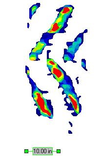
141 Vehicle R4 Axle 1 0% Axle 1 25% Axle 1 80% Axle 2 0% Axle 2 25% Axle 2 80% 126

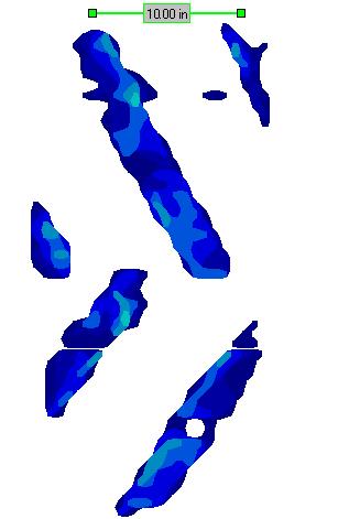
142 Vehicle S3-R5 Axle 1 0% Axle 1 50% Axle 1 80% Axle 2 0% Axle 2 50% Axle 2 80% 127

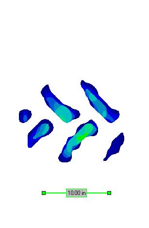
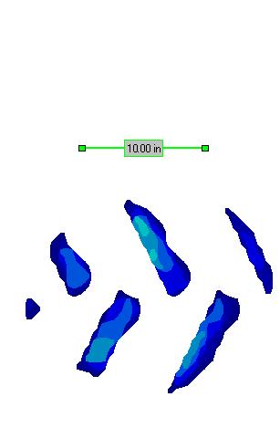
143 Vehicle T1 Axle 1 0% Axle 1 50% Axle 1 80% 128

144 Axle 2 outer 0% Axle 2 outer 50% Axle 2 outer 80% Axle 2 inner 0% Axle 2 inner 50% Axle 2 inner 80% 129

145 Axle 3 0% Axle 3 50% Axle 3 80% Axle 4 0% Axle 4 50% Axle 4 80% 130

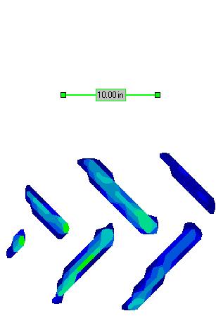
146 Vehicle T2 Axle 1 0% Axle 1 50% Axle 1 80% Axle 2 0% Axle 2 50% Axle 2 80% 131

147 Axle 3 0% Axle 3 50% Axle 3 80% Axle 4 0% Axle 4 50% Axle 4 80% 132

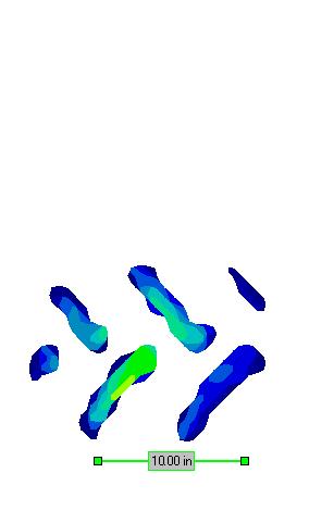
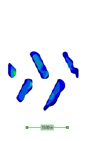
148 Vehicle T3-T6 Axle 1 0% Axle 1 50% Axle 1 80% Incomplete 133

149 Axle 2 outer 0% Axle 2 outer 50% Axle 2 outer 80% Incomplete Axle 2 inner 0% Axle 2 inner 50% Axle 2 inner 80% 134

150 Axle 3 0% Axle 3 50% Axle 3 80% Axle 4 0% Axle 4 50% Axle 4 80% 135

151 Vehicle T4-T7 Axle 1 0% Axle 1 25% Axle 1 80% 136

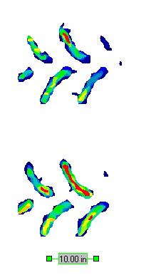
152 Axle 2 0% Axle 2 25% Axle 2 80% 137

153 Axle 3 0% Axle 3 25% Axle 3 80% Axle 4 0% Axle 4 25% Axle 4 80% 138

154 Axle 5 0% Axle 5 25% Axle 5 80% 139

155 Vehicle T5-T8 Axle 3 80% Axle 4 80% Axle 5 80% Axle 6 80% 140

156 Appendix D: Pavement Response Data The figures presented here were taken from Jason Lim s thesis titled, The Effects of Heavy Agricultural Vehicle Loading on Pavement Performance. They are intended to give background information on the data that was collected in the earlier portions of this study. This section provides charts of pavement responses generated by all tested agricultural vehicles compared against the responses generated by the control vehicle Mn80. Only pavement responses at the highest load levels tested for each test season were presented here. For Cell 83, sensors 83AE4 and 83PG4 are presented. For Cell 84, sensors 84LE4, 84TE4, and 84PG4 are presented. Additionally, the pavement responses were plotted against the vehicles wheel path relative to the sensor location. Figure D.1 through Figure D.5 show responses for test during the fall 2008 season. Figure D.6 through Figure D.15 show responses for tests conducted in the spring 2009 season. Figure D.16 through Figure D.25 show responses for tests conducted in fall Figure D.26 through Figure D.28 show responses for tests conducted in spring 2010 and Figure D.29 through Figure D.34 show responses for tests conducted in fall Fall 2008 Figure D.1: Cell 83 angled asphalt strain at 80% load level in fall 2008 for vehicles Mn80, R4, T6, and T7 141

157 Stress [psi] Subgade Stress (83PG4) 80% F Rear axle relative offset [in] Mn80 R4 T6 T7 Figure D.2: Cell 83 subgrade stress at 80% load level in fall 2008 for vehicles Mn80, R4, T6, and T7 Figure D.3: Cell 84 longitudinal asphalt strain at 80% load level in fall 2008 for vehicles Mn80, R4, T6, and T7 142

158 Stress [psi] Figure D.4: Cell 84 transverse asphalt strain at 80% load level in fall 2008 for vehicles Mn80, R4, T6, and T7 Subgade Stress (84PG4) 80% F Rear axle relative offset [in] Mn80 R4 T6 T7 Figure D.5: Cell 84 subgrade stress at 80% load level in fall 2008 for vehicles Mn80, R4, T6, and T7 143

159 Spring 2009 Figure D.6: Cell 83 angled asphalt strain at 80% load level in spring 2009 for vehicles Mn80, S4, S5, R4, and R5 Figure D.7: Cell 83 angled asphalt strain at 80% load level in spring 2009 for vehicles Mn80, T6, T7, and T8 144

160 Stress [psi] Stress [psi] Subgrade Stress (83PG4) 80% S Rear axle relative offset [in] Mn80 S4 S5 R4 R5 Figure D.8: Cell 83 subgrade stress at 80% load level in spring 2009 for vehicles Mn80, S4, S5, R4, and R5 Subgrade Stress (83PG4) 80% S Rear axle relative offset [in] Mn80 T6 T7 T8 Figure D.9: Cell 83 subgrade stress at 80% load level in spring 2009 for vehicles Mn80, T6, T7, and T8 145

161 Figure D.10: Cell 84 longitudinal asphalt strain at 80% load level in spring 2009 for vehicles Mn80, S4, S5, R4, and R5 Figure D.11: Cell 84 longitudinal asphalt strain at 80% load level in spring 2009 for vehicles Mn80, T6, T7, and T8 146

162 Figure D.12: Cell 84 transverse asphalt strain at 80% load level in spring 2009 for vehicles Mn80, S4, S5, R4, and R5 Figure D.13: Cell 84 transverse asphalt strain at 80% load level in spring 2009 for vehicles Mn80, T6, T7, and T8 147

163 Stress [psi] Stress [psi] Subgrade Stress (84PG4) 80% S Rear axle relative offset [in] Mn80 S4 S5 R4 R5 Figure D.14: Cell 84 subgrade stress at 80% load level in spring 2009 for vehicles Mn80, S4, S5, R4, and R5 Subgrade Stress (84PG4) 80% S Rear axle relative offset [in] Mn80 T6 T7 T8 Figure D.15: Cell 84 subgrade stress at 80% load level in spring 2009 for vehicles Mn80, T6, T7, and T8 148

164 Fall 2009 Figure D.16: Cell 83 angled asphalt strain at 100% load level in fall 2009 for vehicles Mn80, Mn102, and R5 Figure D.17: Cell 83 angled asphalt strain at 100% load level in fall 2009 for vehicles Mn80, T6, T7, and T8 149

165 Strain [10-6 ] Stress [psi] Subgrade Stress (83PG4) 100% F Mn80 Mn102 R Rear axle relative offset [in] 0 Figure D.18: Cell 83 subgrade stress at 100% load level in fall 2009 for vehicles Mn80, Mn102, and R5 Subgrade Stress (83PG4) 100% F Mn80 T6 T7 T Rear axle relative offset [in] Figure D.19: Cell 83 subgrade stress at 100% load level in fall 2009 for vehicles Mn80, T6, T7, and T8 150

166 Figure D.20: Cell 84 longitudinal asphalt strain at 100% load level in fall 2009 for vehicles Mn80, Mn102, and R5 Figure D.21: Cell 84 longitudinal asphalt strain at 100% load level in fall 2009 for vehicles Mn80, T6, T7, and T8 151

167 Figure D.22: Cell 84 transverse asphalt strain at 100% load level in fall 2009 for vehicles Mn80, Mn102, and R5 Figure D.23: Cell 84 transverse asphalt strain at 100% load level in fall 2009 for vehicles Mn80, T6, T7, and T8 152

168 Strain [10-6 ] Stress [psi] Subgrade Stress (84PG4) 100% F Mn80 Mn102 R Rear axle relative offset [in] 0 Figure D.24: Cell 84 subgrade stress at 100% load level in fall 2009 for vehicles Mn80, Mn102, and R5 Subgrade Stress (84PG4) 100% F Mn80 T6 T7 T Rear axle relative offset [in] Figure D.25: Cell 84 subgrade stress at 100% load level in fall 2009 for vehicles Mn80, T6, T7, and T8 153

169 Spring 2010 Figure D.26: Cell 84 longitudinal asphalt strain at 100% load level in spring 2010 for vehicles Mn80, Mn102, R6, and T6 Figure D.27: Cell 84 transverse asphalt strain at 100% load level in spring 2010 for vehicles Mn80, Mn102, R6, and T6 154

170 Stress [psi] Subgrade Stress (84PG4) 100% S Mn80 Mn102 R6 T Rear axle relative offset [in] Figure D.28: Cell 84 subgrade stress at 100% load level in spring 2010 for vehicles Mn80, Mn102, R6, and T6 Fall 2010 Figure D.29: Cell 84 longitudinal asphalt strain at 100% load level in fall 2010 for vehicles Mn80, Mn102, and T6 155

171 Figure D.30: Cell 84 longitudinal asphalt strain at 100% load level in fall 2010 for vehicles Mn80, Mn102, and G1 Figure D.31: Cell 84 transverse asphalt strain at 100% load level in fall 2010 for vehicles Mn80, Mn102, and T6 156

172 Stress [psi] Figure D.32: Cell 84 transverse asphalt strain at 100% load level in fall 2010 for vehicles Mn80, Mn102, and G1 Subgrade Stress (84PG4) 100% F Mn80 Mn102 T Rear axle relative offset [in] 0 Figure D.33: Cell 84 subgrade stress at 100% load level in fall 2010 for vehicles Mn80, Mn102, and T6 157

173 Stress [psi] Subgrade Stress (84PG4) 100% F Mn80 Mn102 G Rear axle relative offset [in] 0 Figure D.34: Cell 84 subgrade stress at 100% load level in fall 2010 for vehicles Mn80, Mn102, and G1 158

174 Appendix E: Tekscan (Increased Representative Area Analysis) Table E.1: Tekscan analysis for vehicle T7, Axle 5, Fully Loaded T7Houle7300FullAxle5 Total Area Centroid Centroid Wheel Load x y x(in) y(in) Average Pressure Section x y x (in) y (in) Area (in^2) Radius Load Pressure

175 Section x y x (in) y (in) Area (in^2) Radius Load Pressure

176 Section x y x (in) y (in) Area (in^2) Radius Load Pressure

177 Appendix F: HAVED2011 Users Guide The damage analysis procedure developed in this study has been implemented into a FORTRAN program HAVED2011. To execute the program, the user has to create an input file containing information about the pavement structure, climatic data, layer moduli and loads. The file should be saved in the same directory as the program HAVED2011. To execute the program, the name of the batch file to be run should be typed in the DOS prompt in the same directory where HAVED2011is located: Figure F-1 shows a screenshot with the command line with batch file name a : Figure F-1: Example of HAVED2011 execution After execution, the program will create the following output files: Input_file_name_Tdam.out a file containing the details of damage calculation from 18-kip single axle loads SFdamsum.out a file containing relative AC cracking and rutting damage parameters, as well as SR and DDI values. 162