Hybrid Power System Intelligent Operation and Protection Involving Distributed Architectures and Pulsed Loads

Transcription

1 Florida International University FIU Digital Commons FIU Electronic Theses and Dissertations University Graduate School Hybrid Power System Intelligent Operation and Protection Involving Distributed Architectures and Pulsed Loads Ahmed A. Mohamed Florida International University, DOI: /etd.FI Follow this and additional works at: Part of the Power and Energy Commons Recommended Citation Mohamed, Ahmed A., "Hybrid Power System Intelligent Operation and Protection Involving Distributed Architectures and Pulsed Loads" (2013). FIU Electronic Theses and Dissertations This work is brought to you for free and open access by the University Graduate School at FIU Digital Commons. It has been accepted for inclusion in FIU Electronic Theses and Dissertations by an authorized administrator of FIU Digital Commons. For more information, please contact

2 FLORIDA INTERNATIONAL UNIVERSITY Miami, Florida HYBRID POWER SYSTEM INTELLIGENT OPERATION AND PROTECTION INVOLVING DISTRIBUTED ARCHITECTURES AND PULSED LOADS A dissertation submitted in partial fulfillment of the requirements for the degree of DOCTOR OF PHILOSOPHY in ELECTRICAL ENGINEERING by Ahmed Mohamed 2013

3 To: Dean Amir Mirmiran College of Engineering and Computing This dissertation, written by Ahmed Mohamed, and entitled Hybrid Power System Intelligent Operation and Protection Involving Distributed Architectures and Pulsed Loads, having been approved in respect to style and intellectual content, is referred to you for judgment. We have read this dissertation and recommend that it be approved. Mark Roberts Arif Islam W. Kinzy Jones Armando Barreto Osama A. Mohammed, Major Professor Date of Defense: March 21, 2013 The dissertation of Ahmed Mohamed is approved. Dean Amir Mirmiran College of Engineering and Computing Dean Lakshmi N. Reddi University Graduate School Florida International University, 2013 ii

4 Copyright 2013 by Ahmed Mohamed All rights reserved. iii

5 DEDICATION I dedicate this dissertation to my lovely wife, Yassmin Ali, my mother and my father, Prof. Ali El-Tallawy. Without their patience, understanding, support, encouragement, and most of all love, the completion of this work would not have been possible. iv

6 ACKNOWLEDGMENTS This dissertation would not have been possible without the help, support, resolute dedication and patience of my principal supervisor, Prof. Osama Mohammed, whose passion for success has inspired me to take my own passions seriously, not to mention his advice and unsurpassed knowledge of the various fields of Electrical Power Systems. Prof. Mohammed has always been an endless supply of ideas, guidance, suggestions and useful discussions for me. I am indebted for his enthusiasm, advice, moral as well as financial support and friendship. I am also grateful for the chance he gave to me to work at the Energy Systems Research Laboratory, where I found all the first-class equipment I needed to experimentally verify my results and, where I was developed professionally in an environment where work and engineering ethics are highly respected. I am thankful to Dr. Mark Roberts, Dr. Arif Islam, Professor W. Kenzy Jones and Dr. Armando Barreto for serving on my committee and for their discussions and support. Thanks are also due to all my colleagues at the Energy Systems Research Laboratory whose discussions, contributions and assistance helped me achieve my research goals. I also owe sincere thankfulness to my family for their love, support and encouragement. I offer my deepest gratitude to my mother for her endless love, tenderness and care and for my father, Prof. Ali Hassan El-Tallawy, for his confidence in me and for his advice, which always brings previously unrecognized aspects of each situation to my attention. I also extend my gratitude to my wife, Yassmin, and my sisters, Rasha and Dina, for their love and support. v

7 ABSTRACT OF THE DISSERTATION HYBRID POWER SYSTEM INTELLIGENT OPERATION AND PROTECTION INVOLVING DISTRIBUTED ARCHITECTURES AND PULSED LOADS by Ahmed Mohamed Florida International University, 2013 Miami, Florida Professor Osama A. Mohammed, Major Professor Efficient and reliable techniques for power delivery and utilization are needed to account for the increased penetration of renewable energy sources in electric power systems. Such methods are also required for current and future demands of plug-in electric vehicles and high-power electronic loads. Distributed control and optimal power network architectures will lead to viable solutions to the energy management issue with high level of reliability and security. This dissertation is aimed at developing and verifying new techniques for distributed control by deploying DC microgrids, involving distributed renewable generation and energy storage, through the operating AC power system. To achieve the findings of this dissertation, an energy system architecture was developed involving AC and DC networks, both with distributed generations and demands. The various components of the DC microgrid were designed and built including DC-DC converters, voltage source inverters (VSI) and AC-DC rectifiers featuring novel designs developed by the candidate. New control techniques were developed and implemented to maximize the operating range of the power vi

8 conditioning units used for integrating renewable energy into the DC bus. The control and operation of the DC microgrids in the hybrid AC/DC system involve intelligent energy management. Real-time energy management algorithms were developed and experimentally verified. These algorithms are based on intelligent decision-making elements along with an optimization process. This was aimed at enhancing the overall performance of the power system and mitigating the effect of heavy non-linear loads with variable intensity and duration. The developed algorithms were also used for managing the charging/discharging process of plug-in electric vehicle emulators. The protection of the proposed hybrid AC/DC power system was studied. Fault analysis and protection scheme and coordination, in addition to ideas on how to retrofit currently available protection concepts and devices for AC systems in a DC network, were presented. A study was also conducted on the effect of changing the distribution architecture and distributing the storage assets on the various zones of the network on the system s dynamic security and stability. A practical shipboard power system was studied as an example of a hybrid AC/DC power system involving pulsed loads. Generally, the proposed hybrid AC/DC power system, besides most of the ideas, controls and algorithms presented in this dissertation, were experimentally verified at the Smart Grid Testbed, Energy Systems Research Laboratory. All the developments in this dissertation were experimentally verified at the Smart Grid Testbed. vii

9 TABLE OF CONTENTS CHAPTER PAGE 1. Introduction Types of DC Distributed Power System Architectures... 3 Centralized power systems... 4 Modular power systems... 4 Distributed power systems... 5 DC Microgrids in Smart Grid Applications... 6 Benefits of DC Microgrid Deployment... 8 Influence of High Penetration of DC Microgrids in Modern Smart Grids Energy savings (MWH) Additional benefits for on-site power generation from DC Sources Obstacles against DC Microgrid Deployment Information and education program for construction industry and code officials Codes and standards Federal tax law Business Model and Energy Pricing Renewable Electricity Standard Factors Influencing the AC- versus DC-Distribution Debate Reliability and Un-interruptible Power Supplies (UPS) Alternative Energy Sources Loads Protection Cables Voltage Transformation Examples of Existing DC Power Systems Data Centers Spacecraft Telecommunications Feasibility of AC/DC Distribution Systems Problem Statement Research Objectives Originality of the Research Significance of the Research Organization of Dissertation Hybrid AC/DC Smart Grid Testbed System Description DC Bus and DC Microgrid Implementation AC System Implementation System Real-time Operation DC Microgrid Operation viii

10 AC Grid Operation Integrated Hybrid AC/DC Operation Integration of Renewable Energy Sources into DC Microgrids Energy link Integration Energy Link Integration DC-DC Boost Converter Inductively Coupled Boost Converter Parallel/Series Compensation.Proposed Integration Technique Results and discussion Conventional Boost Converter Results Inductively Coupled Boost Converter Results Parallel/series Compensation Topology Results Grid-Connectivity and Bi-directional Energy Transfer.Modeling, Simulation and Hardware Implementation Microgrid Connectivity DC Bus Voltage regulation Converter Description and Mathematical Modeling Vector Decoupling Technique Bi-directional Energy Transfer Results and discussion DC Bus Voltage Results Bi-directional power flow results LCL-Filter Based Bi-directional Converters Real-Time Load Emulation Reactive Power Controller Active Power Controller Results and Discussion Smart Controller of Power Conditioning Units for Performance Enhancement of Renewable Energy Integration Introduction PV Arrays Characteristics Adaptive Fuzzy-PID Control for PV Systems Supplying Power in DC Form 138 Maximizing the Operating Range Enhancing Transient and Steady State Response Results of the proposed adaptive fuzzy-pid controller Controllers Coordination of Power Electronic Converters for PV Systems Supplying Power in AC Form Steady state performance Dynamic performance Real-Time Energy Management Scheme for Hybrid Renewable Energy Systems in Smart Grid Applications ix

11 Energy Management Concept System and Problem Description Data Forecasting Data Collection and Filtering Online PV Data Modeling Non-Linear Regression Modeling for Wind and Load Data Model Evaluation Indices Results of the Mathematical Model The Energy Commitment Problem Case 1-Power Surplus Case 2-Power Deficiency Proposed Fuzzy System Model Results and Discussion Real-Time Energy Management Algorithm for Mitigation of Pulsed Loads in Hybrid Microgrids Pulsed Loads PV and Load Data Forecasting Non-linear Regression Modeling and Model Evaluation Indices Mathematical Modeling Results Hybrid Storage System Real Time Energy Management Algorithm Super Capacitors are always Fully Charged to Mitigate Possible Pulsed Loads Li-ion Batteries have Enough Energy to Help Super Capacitors Mitigate Pulsed Loads Normal Loads on the Smart Microgrid are Supplied Using PV System Operating at its Maximum Power Point Any Load Deficiency on the Microgrid is Supplied from the battery if it is during a Peak Period or from the Grid if it is an Off-peak Period Fuzzy Agent Involvement during Power Deficiencies Results and Discussion Cost Minimization Pulsed Load Mitigation System Performance under Auxiliary Generator Outage Stability and Security Analyses of Hybrid AC/DC Power Systems Involving Pulsed Loads Hybrid AC/DC Power System Stability Power System Security System Security against Contingency Conditions Effect of Storage Distribution on System Dynamic Security Real-Time Energy Management Algorithm for Plug-In Hybrid Electric Vehicle Charging Parks Involving Sustainable Energy x

12 EVs Batteries Charging/Discharging Coordination Charging Park Architecture Modeling System Uncertainties Online PV Modeling PHEVs Arrival and Departure Times PHEVs Energy Demand Real Time Energy Management Algorithm PHEVs Charging Priority Levels Real-Time Decision Making Process Daily Load Curve Consideration Results and Discussion All PHEVs are connected to Bus PHEVs are distributed equally among 5 Buses PHEVs are distributed equally among 10 Buses Design and Protection of Distributed DC Power System Architectures Laboratory Setup System Design System Layout Uncontrolled Rectifier Design Filter Design Photovoltaic Generation and Battery Storage DC-DC Converter Design System Control and Operation Master-Slave (Communication-Based) Control Mode Droop Control Mode Heavy Load Mitigation Mode Operational Results and Discussion Protection Design and Equipment Fault Analysis and Coordination Scheme AC Side Faults DC Side Faults Distributed Architectures Implementation AC Radial Distribution Medium Voltage DC Distribution AC Zonal Distribution DC Zonal Distribution Response to Pulsed Loads Conclusions and Future Work Conclusions Recommendations for Future Work LIST OF REFERENCES xi

13 13. APPENDICES VITA xii

14 LIST OF TABLES TABLE PAGE 1.1 Photovoltaic Panel Types and Their Corresponding Efficiency Transmission Line Parameters Synchronous Generators Parameters DC Microgrid Parameters Parameters of different prototype systems used for simulation and experimental results Comparison between the DC-DC boost converter and the modified configuration Comparison between the inductors in LCL-filter and L-filter based converters, physical properties Comparison between LCL-filter and L-filter based converters, electrical quantities Kp, Ki and Kd optimal values at input voltage of 110 V and different output current ranges Specifications of PB 175 solar panels Efficiency and THD of the various components of the system Parameters of the system under study Fuzzy rules Security constraints A list of the events studied Dynamic security analysis summary Parameters of the duration time probability distribution Charging rate for different charging levels Fuzzy Rules xiii

15 9.4 A summary of the results using RTEMA in 69-bus radial distribution feeder in different cases System Parameters xiv

16 LIST OF FIGURES FIGURE PAGE 1.1 DC Distribution Architectures Solar Cell circuit model P-V and I-V characteristics of solar panels Solid oxide fuel cell system Use of existing cables in DC systems A Hybrid AC/DC power system DC network schematic interconnected to AC side and DC source and load emulators Output voltage from the fuel cell emulator A block diagram of the DC-DC boost converter controller A block diagram of the Bi-directional battery charger controller Output power of the dynamic load emulator Overall power system schematic and single line diagram of the implemented setup A flow chart of one of the real-time algorithm used to manage the charge/discharge process of the batteries Performance of the various components of the DC microgrid corresponding to step changes in the power reference. (a) shows the DC bus voltage (v dc ), (b) the rectifier current (i r ), (c) the bi-directional current (i bdc ), (d) the PV output current (i pv ), (a) Active power and (b) Reactive power of generators during load increase in manual control mode (a) Active power and (b) Reactive power of generators during load increase in automatic control mode Performance of the integrated hybrid AC/DC microgrid corresponding to step change in the load demand reference. (a) shows the load, DC and AC active xv

17 power share, (b) the load, DC and AC reactive power share, (c) the frequency of the AC bus, (d) the voltage of the AC and DC buses Current and voltage waveforms, and their THD after 10 s. (a) shows the PCC current and voltage waveforms, (b) the inverter side current and voltage phasors, (c) the current and voltage THD Current and voltage waveforms, and their THD after 70 s. (a) shows the PCC current and voltage waveforms, (b) the inverter side current and voltage phasors, (c) the current and voltage THD Overall View of the Hybrid AC/DC Smart Grid Testbed The DC ZEDS under study, (Type 1 converter) is the one under study in this paper. (Type 2 converter) can be a conventional controlled DC-DC boost converter Controlled boost converter for fuel cells integration into a DC ZEDS Circuit configuration during different states of the power electronic switch: (a) During turn ON state (0 < t DTs), (b) During turn OFF state (DTs < t T) The proposed Inductively Coupled Boost Converter topology for fuel cells integration into a DC ZEDS The ON and OFF states of the DC-DC converter with output L-filter described in subsection 3.3: (a) (0 < t DTs) and (b) (DTs < t T) The proposed Parallel/series Compensation Topology for fuel cells integration into a DC ZEDS: (a) circuit and control diagram, (b) block diagram describing the connection The ON and OFF states of the DC-DC converter with compensating fly back converter described in subsection 3.4: (a) (0 < t DTs) and (b) (DTs < t T) Bode plots of the controllers designed for the proposed topologies: (a) a block diagram of the controller, where, i is 1 for the inductively coupled boost converter and 2 for the parallel/series compensation topology, (b) bode plot for the open and clos Controlled conventional boost converter for fuel cells integration into a DC ZEDS: (a) simulation results, (b) experimental results (same scale) Results for (Inductively Coupled Boost Converter) discussed in section 3.4: (a) simulation results, (b) experimental results (same scale) The application of (Inductively Coupled Boost Converter) for power sharing among different sustainable energy sources connected to a common DC bus xvi

18 3.12 Power sharing response to a step change in the power reference, (a) simulation results, (b) experimental results (same scale) Power sharing response to a step change in the load, (a) simulation results, (b) experimental results (same scale) Experimental results for the performance of (proposed parallel/series compensation technique) Voltage at both microgrids and power flowing between them when both microgrids have the same voltage level, black line is the reference and grey line is the actual response Voltage at both microgrids and power flowing between them when both microgrids have the different voltage levels, black line is the reference and grey line is the actual response The implemented three phase SPWM rectifier; (a) circuit diagram, (b) singlephase equivalent A block diagram of the vector-decoupling control implemented on the controlled rectifier Circuit diagram of the implemented three phase bi-directional AC-DC/DC-AC converter A block diagram of the vector-decoupling control implemented on the bidirectional converter Voltages of the grid connected to the DC microgrid under study; (a) experimental results, (b) simulation results Line currents during steady state operation; (a) experimental results, (b) simulation results Unity power factor operation of the proposed controlled rectifier; (a) experimental results, (b) simulation results (AC current factorized by 10) Controlled rectifier s response to a load step change; (a) experimental results, (b) simulation results Controlled rectifier s response to a change in the output voltage; (a) experimental results, (b) simulation results Controlled Bi-directional response to DC current reference change from 1-3 A, (a) experimental results, (b) simulation results (AC current factorized by 10) Controlled bi-directional converter response to DC current reference change xvii

19 from 3-1 A; (a) experimental results, (b) simulation results (AC current factorized by 10) Controlled bi-directional converter response to DC current reference change (- 3)-(-1) A; (a) experimental results, (b) simulation results (AC current factorized by 10) Controlled bi-directional response to DC current reference change (-3)-(3) A; (a) experimental results, (b) simulation results (AC current factorized by 10) Controlled bi-directional comverter response to DC current reference change (3)-(-3) A; (a) experimental results, (b) simulation results (AC current factorized by 10) Harmonic analysis of the grid currents Results for the LCL-filter based converter Results for the L-filter based converter Circuit diagram of the developed dynamic load emulator A block diagram of the dynamic emulator controller Dynamic load emulator steady state response when P is set to 1000 Watts and Q is set to zero Dynamic load emulator steady state response when Q is set to 1000 Vars and P is set to zero Dynamic load emulator steady state response when P is set to 1000 Watts and Q is set to 1000 Vars Dynamic emulation of a load varying at low frequency Dynamic emulation of a short term pulsed load Dynamic emulation of a load with reactive power varying at a high frequency Dynamic emulation of a load with its active/reactive power varying at a high frequency THD of the line current Efficiency of the dynamic load emulator Power and current versus voltage characteristics of a PV panel xviii

20 5.2 A typical stand-alone PV system Load step change voltage response for (a) conventional PI controller, 110 V input voltage and (b) proposed controller, 110 V input voltage A block diagram of the fuzzy controller utilized in this chapter Membership functions for: (a) output current, (b) PV voltage Membership functions for: (a) Kp gain, (b) Ki gain and (c) Kd gain Surface plots of (a) the Kp gain, (b) the Ki gain and (c) the Kd gain Load step change voltage response for conventional PID controller Block diagram of the proposed controller Proposed adaptive controller load step change, 100 W-500 W, response and controller parameters variations Proposed adaptive controller load step change, 500 W-100 W, response and controller parameters variations Traditional PI controller response to a load step change (a) from 100 W to 500 W, (b) from 500 W to 100 W A photograph showing the experimental setup used in this paper Experimental results showing the response of various controllers to a load step change from 220 W to 1 kw: current (1.1 A/div) and voltage (65 V/div), (a) proposed adaptive PID controller, (b) proposed controller (with Kd gain set to zero), (c) traditional PI controller (a) Variations of THD versus V dc, optimum V dc =210 V, (b) Steady state stability of the system with respect to DC link voltage Results for voltage and current variations during switching of a 220 W load for the fast controller: (a) simulation, (b) experimental Results for voltage and current variations during switching of a 220 W load for the slow controller: (a) simulation, (b) experimental Results voltage and current variations during switching of a 265 W load for the fast controller: (a) simulation, (b) experimental Results for Voltage and current variations during switching of a 265 W load for the slow controller: (a) simulation, (b) experimental xix

21 6.1 Schematic diagram of the investigated system Bi-directional converter response to a step change in the DC current reference from -4 to 1 A. (a) DC current, i dc (4 A/div, 10 ms). (b) DC voltage, v dc (1000 V/div, 10 ms). (c) AC phase voltage, e a (30 V/div, 10 ms). (d) AC current, i a (5 A/div, 10 ms PV filtered actual data, support vectors (dots) versus modelling (surface) data for one year Wind filtered actual data, support vectors (dots) versus modelling (surface) data for one month Load demand filtered actual data, support vectors (dots) versus modelling (surface) data for one year Battery power as a function of its SoC when there is an excess in power within the OFF-peak period Battery power as a function of its SoC when there is an excess in power within the peak period Battery power as a function of its SoC when there is a deficiency in power within the peak period Membership functions of different variables of the fuzzy controller: (a) and (b) show the membership functions of the two inputs to the Fuzzy system. Whereas, (c) shows the membership functions of the output variable Case study 1, dynamic operation of the proposed algorithm in a one day-period Case study 2, dynamic operation of the proposed algorithm in a one day-period Performance of the energy commitment algorithm close to and around the peak period Performance of the energy commitment algorithm for a 10-day interval Battery/SC hybrid storage system: (a) Passive hybrid, (b) Active hybrid A flow chart of the developed energy management algorithm Operation of the system for a 24 hours interval, while applying Algorithms 1 and The example system simulated in this chapter Operation of the system for a 24 hours interval, while applying Algorithms 1 and xx

22 Active power of the pulsed loads and the power sharing among AC generators, super capacitor and full-charged battery (Case 1) Voltage amplitude of AC buses during pulsed-loads (Case 1) Loading of the main generators during pulsed-loads (Case 1) System AC side frequency during pulsed-loads (Case 1) Active power of the pulsed loads and the power sharing among AC generators, super capacitor and half-charged battery (Case 2) DC bus and battery voltage during pulsed-load (Case 2) Voltage amplitude of AC buses during pulsed-loads (Case 1) System AC side frequency during pulsed-loads (Case 2) Loading of main generators during pulsed-loads (Case 2) Power-Delta Curve for main generator during Pulsed Load (Case 1) Power-Delta Curve for main generator during Pulsed Load (Case 2) Active power of the pulsed loads and the power sharing among AC generators, super capacitor and full-charged battery (Outage of ATG1 at t=1s) System AC side frequency and voltages during pulsed-loads with half-charged battery (Outage of ATG1 at t=1sec) Active power of the pulsed loads and the power sharing among AC generators, super capacitor and half-charged battery (Outage of ATG1 at t=1s) Effect of source voltage and internal resistance on maximum power point in DC systems P-V curves of DC networks A single line diagram of the hybrid AC/DC system studied in this chapter Response of the hybrid power system to the pulsed load when the system is encountering no contingencies Response of the hybrid power system to the pulsed load when the system is subjected to cable 1-2 outage xxi

23 8.6 Response of the hybrid power system to the pulsed load when the system is subjected to cable 1-2 outage Response of the hybrid power system to the pulsed load when the system is subjected to MTG2 outage Response of the hybrid power system to the pulsed load when the system is subjected to MTG2 outage with distributed storage Response of the hybrid power system to the pulsed load when the system is subjected to ATG2 outage Response of the hybrid power system to the pulsed load when the system is subjected to PMSM outage Response of the hybrid power system to the pulsed load with the storage connected at zone 1 (with the pulsed load) Response of the hybrid power system to the pulsed load with the storage connected at zone 4 (far from the pulsed load) Response of the hybrid power system to the pulsed load with the storage distributed between zones 1 and Response of the hybrid power system to the pulsed load with the storage distributed among zones 1, 2, 3 and Response of the hybrid power system to the pulsed load with no battery storage One-line diagram showing a lumped model of the PHEVs charging park power system PDF of the parking duration time of PHEVs (D t -A t ) PDF of the miles driven daily for PHEVs PDF of the daily power needed by PHEVs A flow-chart showing the developed RTEMA Bus Radial Distribution Test Feeder Florida s normalized summer and winter daily load curves Bus daily voltage profile with no PHEVs for summer load Bus daily voltage profile with no PHEVs for winter load xxii

24 9.10 PHEVs daily load profile in with no optimization and different optimization objectives Daily voltage profile with no RTEMA for summer load Daily voltage profile with no RTEMA for winter load Daily voltage profile with RTEMA considering energy function for summer load Daily voltage profile with RTEMA considering energy function for winter load Daily voltage profile with RTEMA considering energy function and summer load curve Daily voltage profile with RTEMA considering energy function and winter load curve A Schematic diagram of the developed laboratory based testbed setup A circuit diagram of each zone Hardware components developed for the implemented system: (a) uncontrolled rectifier, (b) AC filter, (c) DC filter, (d) controlled DC-DC boost converter, (e) AC measurement and protection box, (f) DC measurement and protection box and (g) load emulator DC output currents from each of the four zones corresponding to a total load of 1.9 kw (initial), then a step change in the load to 3.8 kw (1.5 A/div, ms/div) AC currents and DC voltage response to a total load of 1.9 kw (initial), then a step change in the load to 3.8 kw (Vdc: 300 V/div, 33.3 ms/div, Ia,b,c: 2 A/div, 33.3 ms/div) DC output currents response from each of the four zones corresponding to a set of step changes in the current reference (2 A/div, 0.2 s/div) AC voltages and DC voltage response to a set of load step changes (Vdc: 300 V/div, 33.3 ms/div, Va,b,c: 70 V/div, 33.3 ms/div) A schematic diagram of the system under study; (a) layout of the system and faults locations, (b) snubber circuit Line to Line fault at FP1; (a) current in phases A and B 180 apart and crossing limit of 1.23 p.u, (b) line to ground voltage going less than undervoltage limit of 0.75 p.u xxiii

25 10.10 Line to Ground fault at FP1; (a) current crossing the limit of 1.23 p.u, (b) line to ground voltage going less than undervoltage of 0.75 p.u Pole to Pole fault at point FP2; (a) derivative of the DC current, (b) DC bus voltage Coordination between the faults at FP2 and FP4; (a) derivative of the DC current, (b) derivative of the bus voltage The developed reconfigurable testbed Radial AC distribution Medium voltage DC distribution Zonal AC distribution Zonal DC distribution Radial AC architecture response Medium voltage DC architecture response Zonal AC architecture response Zonal DC architecture response xxiv

26 Chapter 1 : Introduction Currently, there is a national call for improving the current electric power systems into smart and more distributed operational grids. The goals of having a smart grid include improved reliability, security, increased efficiency, sustainability and most importantly, increased penetration of renewable energy and storage resources. These goals can all be realized using hybrid AC/DC power systems involving DC distributed architectures, or microgrids [1]-[3]. A DC microgrid is a perfect place to integrate renewable energy, such as photovoltaic (PV), fuel cells (FC) or even wind [4]-[9]. It is also the place where battery storage can be implemented with the fewest number of conversion stages [10], [11]. Moreover, with this exponentially increasing penetration of electronic loads, variable frequency machine drives and other loads working with DC power, utilizing a DC bus and/or a DC distribution system architecture will have a significant impact on the overall system efficiency [4]. However, the idea of reconsidering DC microgrids has only been researched during the past few years mostly either from a perspective of trying to convince others of the feasibility of reconsidering DC systems, or trying to retrofit today s AC technologies to DC systems. A few articles also investigated the feasibility of DC superconducting DC networks [12], [13]. In this dissertation, an initiative is taken to have a wider look at the DC microgrid while operating within a smart grid, where wide area measurement, protection, and control are activated. The element of energy management, which is a key target of smart grids, is investigated in this dissertation. An intelligent energy management algorithm could play a vital role in the solution of many power system problems. For instance, an algorithm aiming at shifting the demand to off-peak hours can significantly decrease the burden on 1

27 the utility grid while decreasing consumers costs. Furthermore, energy management cannot be just an optional privilege in the near future with an expected vast increase in the number of plug-in hybrid electric vehicles. The focus is also on the technologies and controls needed to implement an efficient intelligently-operated hybrid AC/DC microgrid. The debate of AC versus DC distribution is historical and as old as the evolution of the first commercial power systems themselves [14], [15]. This debate, which took place in the nineteenth century and was mostly led by the biggest two electrical companies at that time: Edison s and Westinghouse s companies, was significantly inflamed by the fact that the machines invented at that time were DC machines. AC systems, on the other hand, allowed the transfer of power for long distances. One of the first commercial applications of electrical power was arc lighting systems that were launched in the beginning of the nineteenth century. These lighting systems were supplied using batteries, which limited the practicality of these systems. However, in the 1850s, these lighting systems were made much more practical using dynamos as electrical power supply. Therefore, a single-phase 3.5 kv AC system was developed. In the meantime, Thomas Edison claimed in 1878 that he was capable of building a better lighting system than the arc lighting one; a system that would require less maintenance and could be used both indoors and outdoors. Since Edison was interested in building a power system that would work for machines as well as the incandescent lighting system he invented, he developed a low voltage DC distribution system. Edison s first low voltage system was launched in Pearl Street, downtown Manhattan, New York and covered around one square mile. However, this system had a major drawback, which 2

28 is the limited distance of feeders due to the low voltage. In 1885, George Westinghouse incorporated the patents of Goulard and Gibbs AC transformers with his company and started to build a power system, which utilized both high voltage transmission and low voltage distribution. The number of these AC power systems exceeded the number of DC power systems. In 1887, Nekola Tesla, a former Edison employee, sent a number of patent applications for his poly-phase AC power systems including two-phase induction machines. Westinghouse bought Tesla s patents to his company, hired him and worked on developing poly-phase AC power systems. Consequently, the first poly-phase AC power system that was used to supply both light and machines was launched in Chicago in The first large-scale long distance power transmission was built between Niagara Falls and Buffalo (26 miles) in November Westinghouse together with General Electric developed this power system that transmitted the power in AC form using a three-phase high voltage 10.7 kv. This voltage was transformed down into 440 V for distribution. Moreover, for loads requiring DC power, such as street cars, 550 V DC was obtained using rotary converters. Although the use of AC power systems increased at the beginning of the twentieth century, some DC power systems remained in operation. The last residential DC distribution system was converted into AC in the mid-1970s. Types of DC Distributed Power System Architectures DC power system architectures can be generally categorized into centralized power system, modular power system, and distributed power system (DPS), as shown in figure 1.1. [16] 3

29 Multiple Converters V in Single Converter V 1 V 1 V V 2 V 2 in V 3 V 3 (a) (b) Front-End Converter Bus Local Converter V 1 V in V 2 V 3 (c) Figure 1.1 DC Distribution Architectures Centralized power systems Centralized power systems utilize a single power conversion stage located in one physical location in the system, while multiple outputs are generated and bussed to the various loads. In centralized power systems, all the power processing technologyincluding thermal management are located in a single box that can be designed, subcontracted, or purchased as a stand-alone item. However, this system often fails to provide adequate performance for new generations of electronic equipment. Modular power systems Modular power systems utilize multiple power conversion stages or converters that are located in one location in the system, usually far away from the load. Voltages and currents can be combined to meet load requirements, when higher power is needed. The 4

30 modular power system is particularly suited for high power design. High power is achieved by paralleling multiple small power stages in a single package, producing the physical equivalent of a single large device. This way, power modules are easily standardized and traditional low-power converter design techniques can be used. Distributed power systems Distributed power systems, usually employing the modular design technique, incorporate the advantages of modular power systems. However, all outputs of the frontend converters go to the intermediate bus by paralleling technology. Its basic characteristics are: Multiple power conversion stages and/or converters can be in different locations. Intermediate voltage is bussed around the system. Multiple DC-DC converters located at the point-of-use are used to provide the local voltage. The major disadvantages of centralized power systems and modular power systems can be eliminated by introducing distributed power process technologies. Moreover, there are some merits that can be achieved using distributed power system architecture. These advantages include facilitating thermal management and packaging associated with the modular design of the converters, modular size reduction, reduced electromagnetic interference (EMI) and harmonics due to the utilization of converters having their own filter. The modular design and standardization help increase the availability of standardized off-the-shelf modules or designs that could be combined in a variety of ways to meet a specific application. Redundancy, reliability, availability and maintainability are added characteristics since repairing a single converter in a distributed 5

31 system is much easier than repairing the main converter in a centralized architecture. Furthermore, point of load regulation due to having load converters and flexible system structure and layout enable distributed power systems to realize complicated power supply architectures to meet different load requirements. DC Microgrids in Smart Grid Applications Although the term smart grid was given several different explanations and views, certain features of a smart grid seem to be agreed upon. As acknowledged by the Energy Independence and Security Act of 2007, the elements that most characterize the Smart Grid policy goals are as follows [4]: reliability; security; storage; distributed generation energy efficiency; sustainability; renewable inputs IT/communications leverage/full cyber-security load awareness; demand side management; plug-in vehicles lowering unnecessary barriers to achieving the above Through the use of DC microgrids, each of these goals can be promoted, often with reduced cost and with greater effectiveness. Our current utilization of energy exceeds what the national grid in the U.S. and around the world is ready for. This forces us to consider the implementation of DC microgrids, which can optimize the use of electronic devices, electrical storage, and distributed generation. Therefore, the interest in DC microgrids is growing over the past 10 years. The U.S. Department of Energy (DOE), the California Energy Commission (CEC), the Electric Power Research Institute (EPRI), along with several utilities and numerous entrepreneurs and investors seek to upgrade the utility grid s operation through Smart Grid initiatives. In large part, these efforts have 6

32 been aimed towards AC systems which currently exist. Conversely, the present dissertation focuses on improving the efficiency, reliability and security of the implementation of the Smart Grid through the use of DC microgrids. It is also worthy at this introductory stage of the dissertation to put a clear definition of the term microgrid. The DOE and the CEC jointly commissioned a report from Navigant Consulting in 2005 that discussed this very definition. The final report identified two Points of Universal Agreement of what constitutes a microgrid: A microgrid consists of interconnected distributed energy resources capable of providing sufficient and continuous energy to a significant portion of internal load demand. A microgrid possesses independent controls, and intentional islanding takes place with minimal service interruption. These two definitions are valid for both the AC and DC domain. DC microgrids can be deployed in a section of a building (nanogrid), building-wide (microgrid) or even spanning several buildings (minigrid). In the balance of this dissertation, we will refer to these systems as DC microgrids, whatever their scale. All of these grids have the common need to adopt standards to guarantee interoperability. A practical and up-to-date example of the convergence of DC microgrids and Smart Grid is the work of over 100 entities, including companies, universities and other bodies, that have come together in a non-profit organization called the EMerge Alliance to encourage low-voltage DC power standards for device manufacturers and systems integrators. With the recent rise of LED lighting technology, the Emerge Alliance expects the momentum of LEDs as a light source for common lighting applications to continue 7

33 and eventually dominate the market. LEDs typically plug into a 110-volt or 208-volt AC power supply that converts that power to 24-volt DC which is what the light source consumes to make visible light. Not coincidently, 24-volt DC is the first DC power standard promulgated by the EMerge Alliance. While this example demonstrates the potential for DC technology in the lighting market, the EMerge Alliance is devoted to standardizing various types of DC systems, further advancing the convergence of DC microgrids in the Smart Grid. Benefits of DC Microgrid Deployment Electronic devices, such as computers, routers and electronic lights (either fluorescent or LED) represent almost half of the electric load in many buildings today. Moreover, Variable Speed Drives (VFD) are increasingly used for electric motors. A DC environment is found to be a more convenient way to deliver power to these loads in order to assure reliability and redundancy. However, better redundancy is not the only benefit gained by applying DC Networks. DC networks do not need AC to DC conversion for every electronic device, which has a significant impact on the efficiency. Power supplies currently on the market impose losses on the power going to the device, typically 15% to 40%. This range of losses in a DC microgrid can be lowered to 10% to 15% by using a higher efficiency conversion for multiple loads. This topology outperforms the currently existing topologies due to the superior economics of bulk conversion versus converter at every point-of-use [17]-[25]. Incorporating DC microgrids has the benefit of superior compatibility of the DC power with storage of electricity. Grid-scale storage can improve the stability of the grid. It may have prevented several of the blackouts and brownouts that took place in the grid 8

34 over the past several years. However, grid scale battery storage is not practically sensible. Another sensible solution is the utilization of distributed batteries connected to a DC network. The summation of these distributed batteries is equivalent to bulk storage except for the fact that: power from the distant battery would suffer other losses the local battery would not. These include inversion losses (going from the DC in the battery to the AC of the grid), transmission and distribution losses (estimated to be 7 to 11% by the U.S. Department of Energy) and finally rectification losses when it gets to your electronic load. Collectively, these losses could add up to as much as 41% of the energy ultimately delivered to a DC device. These conversion losses and line losses can largely be avoided by use of distributed batteries in a DC microgrid. Another great benefit of DC microgrid is that it facilitates the integration of renewable energy sources that are intrinsically DC sources such as solar PV, small wind turbines, or fuel cells. Furthermore, DC microgrids can simplify and raise the efficiency of how plug-in hybrid electric vehicles (PHEV) and electric vehicles (EV) connect to the grid. A DC microgrid can act like a high-efficiency buffer, optimizing generation and storage and increasing grid reliability. Moreover, because DC power has no phase to match, the connection to the vehicle is simplified, providing a more efficient path to its DC battery. On the system scale, the DC microgrid helps activate the vehicle-to-grid (V2G) and vehicle-to-vehicle (V2V) functionalities and facilitates the energy management of the system. By managing sources and loads at a local level, a DC microgrid can maximize its net surplus of power (output to the grid) or deficit (input from the grid). Some of the burden on the grid can be relieved by utilizing this local management of supply and demand by 9

35 creating a buffer to the grid. Demand Side Management (DSM) when used alone cannot accomplish this advantage as efficiently. However, by using the inherent characteristics of DC productively, this lightening of the burden on the grid becomes a feasible possibility [26]-[30]. Influence of High Penetration of DC Microgrids in Modern Smart Grids The Virginia Polytechnic Institute s Center for Power Electronic Systems (CPES) estimates that by 2010, 80% of all electricity used will pass through power electronic systems. Since this estimate relies on a measure of the current status which is mainly AC, we can confidently assume that these conventional systems could all be improved in terms of efficiency by instituting higher-efficiency conversions of AC to DC networks, instead of converting the AC power at each point-of-use. Energy savings (MWH) As estimated by the Lawrence Berkeley National Laboratory (LBNL), the total amount of energy flowing into external power supplies for electronic devices in the U.S. is approximately 290 TWh/year. However, much of this power is lost as heat the U.S. Environmental Protection Agency (EPA) and the DOE s Energy Star program estimates that one-third to one-half of the power sent to these devices is lost. Ultimately, this means that around TWh/year are currently being lost due to these conversions [4]. While most of the comprehensive national electric power data available is regarding the output from the grid, it does not specific how that power is used. Borrowing largely from the U.S. Energy Information Administration s (EIA) categories and data, we can begin to build an understanding of the energy savings possible through the use of DC microgrids [4]. Where savings are derived from improved power supply efficiency only, 10

36 70% or 75% efficiency is used as an average range for AC power supplies, which is generous given the LBNL estimates, and 90% is used for the bulk high-efficiency rectifier that would be used in a DC microgrid. These rectifiers are currently available in the market. Statistics show that potential percentage savings for the residential sector s addressable load: 25.32%; corresponding reduction in the total U.S. load: 2.98%. Addressable load refers to load that can be connected to a DC microgrid. Potential percentage savings for the commercial building sector s addressable load: 19.03%; corresponding reduction in the total U.S. load: 3.03%. Potential percentage savings for the manufacturing sector s addressable load: 20.00%; corresponding reduction in the total U.S. load: 1.09%. Potential percentage savings for the data center sector s addressable load is 28.00%, which corresponds to the reduction in the total U.S. load of 0.37%. All grid stakeholders would benefit if efficiency improvements were able to have an immediate positive impact on capacity. Using concurrent data for our load analysis, it can be noticed that a lower load would deliver large benefits. For example, the 337 TWh of power generation avoided could have allowed grid operators to shut down or avoid construction of about 75 GW of generating capacity. Since DC microgrids reduce end-use loads and facilitate on-site generations, loads on the transmission and distribution system can be significantly reduced. Other longdistance high-voltage DC transmission schemes are outside the scope of this dissertation. It is interesting to note, however, that short high-voltage DC power lines do regularly operate between large service territories of the grid so that these large synchronized pools of AC power can stay connected to each other without the burden of precisely matching the phase of their neighbor. This buffer is important when a large section of the grid is 11

37 brought down for any reason. With DC connections to its neighboring grid territories, coming back on-line is easier when the reviving generator does not have to synchronize with a connected systems precise phase. Additional benefits for on-site power generation from DC Sources A benefit of more efficient DC microgrids is that less heat is produced inside buildings. Due to avoiding cooling loads, as in the data center application, electrical efficiently as much as double the amount. Also noted should be the fact that multiple DC power inputs can easily be integrated into the DC microgrid, which is not the case in AC systems where phase matching is required. Also observed is an extended efficiency to batteries, small wind turbines, fuel cells, and variable speed DC generators. The latter has great potential in that they could respond in near real time to increased load demand, providing more battery-like surge capacity. Combining multiple inputs raises the likelihood that several different fuels could be used at the building site, which increases the intrinsic security of the system. Obstacles against DC Microgrid Deployment Currently, utility regulatory practices and federal environmental law in many states do not recognize the full societal value of energy efficiency and renewable energy investments in general, or particularly of DC microgrids. Our current regulatory framework holds systemic flaws which are well-recognized. They include the failure to internalize the social costs of greenhouse gas emissions; a price on carbon and other GHGs will increase the cost of fossil fuel generation and thus make both energy efficiency and zero-carbon renewable generation more cost-effective. To go even further, utility profits from volume of sales are not decouples by many state utility commissions, 12

38 leaving in place substantial disincentives for utilities to encourage energy efficiency and distributed generation if they decrease utility demand. Information and education program for construction industry and code officials Having good communications about the benefits of DC microgrids is essential. The time-of-use (TOU) pricing have helped people appreciate the electricity in its complexity. Likewise, the awareness of environmental issues, such as carbon emissions and global warming, have piqued the interest of power industry professionals and prompted legislation to address these issues. These facts highlight the need for an organized effort to disseminate information about the benefits DC microgrids offer. Some of this work has already begun by the EMerge Alliance through outreach to utilities, universities, the electrical trades and other interested parties. State and local governments, as primary regulators for buildings, will find that conversion to a DC microgrid system provides a cost-effective method to further energy efficiency goals. Codes and standards The National Electric Code (NEC) does not cover DC power installations below 600-volts DC, so that DC power is accommodated under rules that govern either AC or DC power systems of the same voltage. For instance, for the insulation and shielding requirements for wires carrying electricity under 600 volts. While often not prohibited, a lack of references to DC can give both electricians and companies reason for concern. Well established sections of the code in place for decades have defined the 48-volt DC domain that was once ubiquitous as the voltage in plain old telephone service (POTS). Twenty-four volt DC has had no such history, but systems operating below 30-volts DC, which strictly limit current to under 100 volts-amps are designated Class 2, denoting 13

39 them as intrinsically safe from shock or fire hazard, which is an obvious advantage. The 24-volt DC standard promoted by the EMerge Alliance is in this category. That effort, coordinated with NEC committees input and guidance, will spread the word, but a timely roll-out would benefit greatly from some coordinated efforts from interested areas of the government and standards bodies such as National Institute of Science and Technology (NIST), the American National Standards Institute (ANSI), the National Electrical Manufacturers Association (NEMA), the U.S. Department of Energy, and its system of National Laboratories and Technical Centers. Federal tax law Tax credits and other incentives for energy efficiency, renewable energy and other low- or zero-carbon technologies are provided by federal tax law. However, these incentives fail to provide any significant financial benefit for DC microgrid technology, even though these microgrids can provide extensive savings in energy use and result in large GHG emissions reductions [4]. Business Model and Energy Pricing Implementing DC microgrids is accompanied by some energy pricing issues, the first being Conventional Utility Regulation. The customary electric utility regulatory model is cost-of-service regulation of a vertically integrated power supplier, who maintains a monopoly in local retail. Since this model is still customary in relatively half of the USA, the DC microgrid system (i) is end-user-owned, (ii) is behind-the-meter, and (iii) supplies no output back to the grid, and so the DC microgrid system does not prevent issues under this regulatory model. It is simply another way for the customer to internally distribute power that was purchased from the utility supplier. However, if at least one of the three 14

40 conditions are not being met, regulatory barriers (exploitable by incumbent utilities) can retard deployment of these systems, absent regulatory accommodation to this new technology. One example of such regulatory barriers is third-party systems. One of the appealing models for large-scale DC microgrids is a system owned by a third party this system buys AC power from the utility, and resells it to individual users after it was converted to DC. Two important questions are raised under conventional utility regulation. First, is regulation of the utility sale to the system operator a wholesale sale done by FERC under the Federal Power Act, instead of getting regulated by a state utility commission under state law as a retail sale? Secondly is the question of whether the sale to the end-user is a retail sale that contravenes the utility s retail monopoly. There is not a clear answer to either of these two questions, mostly because the answer is relying on unpredictable FERC precedent relating to submetering, and whims of state law on exclusive retail service areas. Since answering these questions from case to case takes both time and money, the most efficient answer would be a federal statutory solution. One way to do this would be to exempt utility sales to third-party DC microgrid systems from wholesale regulation under the Federal Power Act, based on the state s regulating the utility sale to the third-party microgrid operator, allowing the operator to resell to end-users, and making sure that the utility s rates to the microgrid are not discriminatory. Another example of regulatory barriers which can slow down deployment of DC microgrids is sales back to grid. A benefit of a DC microgrid is the ability to collect DC generations, such as distributed renewable sources, and to sell it back to the grid after it is converted to AC; however the sale to the grid is a wholesale sale and usually falls subject 15

41 to wholesale rate regulation under the Federal Power Act (FPA), unless the Public Utility Regulatory Policies Act (PURPA) exempts it. PURPA typically exempts smaller renewable power generation from regulation under the FPA, but large renewable systems over 20 MW and other local generation like fuel cells and small turbines are not exempt from FPA regulation, effecting the sales of their power to the grid. Also required by PURPA is that utilities purchase the output of qualifying facilities. But, large barriers exist both on a state s ability to require purchase at rates above avoided cost and on the utility s federal law obligation to purchase from these facilities. In major competitive wholesale markets (such as PJM, NY ISO, ISO New England), FERC rules have dismissed utilities of their purchase obligations. Where it exists the federal purchase obligation is limited to the cost the utility would have incurred if it had generated the power itself or purchased it elsewhere, as determined by the state utility regulatory commission. Avoided cost is mostly under retail rates and may not be sufficient enough to support many types of renewable generation. There is also another issue related to a state s authority to require utilities to pay higher than- avoided-cost rates: FERC precedent from 1995 purports to preempt certain state rules requiring utilities to pay qualifying facilities rates in excess of avoided cost. To the extent these rules raise a problem for DC microgrids, they can be dealt with, at least in part, by changes in federal law that (1) permit these systems to sell output at avoided cost rates without regard to size, and (2) give states clear authority to require above avoided-cost rates. (b) DC Microgrids in Restructured Electric Power Markets. In much of the U.S., electric power regulation was restructured to allow retail competitions. DC microgrids face fewer issues in the markets than in cost-of-service areas. While their sale of AC power by a utility or 16

42 other seller may be subject to FERC regulation, the resale of DC power to end-users will not raise questions under exclusive services area laws (which no longer apply). However, sales back to the grid in restructured markets raise similar issues to those discussed in retail cost-of-service markets. A feed-in tariff is a standing offer by a utility to purchase the output of a renewable generator at a fixed or formula rate. A feed-in tariff applicable to DC microgrid renewable generation sold into the grid could significantly improve the economics of these systems. PURPA s avoided cost purchase obligation, discussed above, represents one form of a feed-in tariff albeit a complicated one because in many circumstances it requires a case-by-case determination of the utility s avoided cost. A more useful feed-in tariff arrangement would entail a standardized rate set on the basis of the incentive necessary to deploy the resource rather than on the basis of the purchasing utility s avoided cost. However, this type of tariff is not permissible under federal law if it sets a rate above avoided cost, and a significant question was raised as to whether it is permissible under state law, as we note in the discussion above. Clarifying that PURPA does not preempt higher than avoided cost feed-in tariffs should provide grounds for states to move forward with innovative feed-in tariff proposals, which could benefit DC microgrids and other renewable systems. In addition, feed-in tariffs should be designed to permit DC microgrid renewable generation to receive feed-in tariff credit for its entire renewable output, whether or not consumed within the DC microgrid. In return, the DC microgrid would pay the utility s retail rate for its entire internal load. This type of arrangement allows the DC microgrid to take advantage of the feed-in tariff for its full renewable output without incurring conversion losses that would be necessary if it 17

43 physically delivered its full output to the grid and physically supplied its full internal load from the grid. An alternative to third-party ownership of large scale DC microgrids is utility ownership of the microgrid. This model could be an effective means of deploying systems that sell DC power from a multi-building network to multiple end-users, particularly in states that have exclusive retail service territory laws. If the incumbent utility is the retail seller, then no retail service exclusivity issue arises; however, the DC microgrid service must still be authorized either under the general terms of the state s utility laws or by action of the state regulator. A more important issue is whether the utility will provide a useful and cost-effective DC microgrid service to end-users and whether the public is better served by having competitive offerings from a number of prospective microgrid operators. Renewable Electricity Standards There are current proposals for a Renewable Electricity Standard (RES) which necessitate a minimum percentage of renewable energy resources each year to be purchased or generated by retail electric utilities. Clean renewable energy generators are given tradable renewable energy credits (RECs). Utilities may produce renewable energy from their own facilities, or they may purchase RECs for use for compliance purposes. Saving in electricity from energy efficiency could also be used for compliance purposes. Full credit for renewables delivered into a DC microgrid system could be provided by the RES as currently formulated, but it is yet unclear what the treatment of the efficiency gains from these systems is. There is a need for an RES provision particularly formed to DC microgrids which provides explicit credit for efficiency gains (from lower conversion 18

44 losses) in order to solve any issues related to electricity savings being computed through use of the general provisions. The DOE could be directed to determine electricity savings by rule through such a provision, based on the difference between losses due to conversion for the average AC system minus demonstrated lowered losses due to conversion for the DC microgrid. Factors Influencing the AC- versus DC-Distribution Debate Reliability and Un-interruptible Power Supplies (UPS) Our growing desire for reliable information technologies requires uninterruptible power supplies. Each such supply must provide dc bus battery storage, which can continue to supply an application with power during unplanned ac outages. The efficiency of this type of systems, which is a must in data center applications, would significantly increase if it is DC-based [31]. Alternative Energy Sources There is currently a great leap towards the utilization of alternative energy sources, such as photovoltaic panels, fuels cells, wind turbines and microturbines. Therefore, it is highly expected that the penetration level of these sources will keep increasing in future. Some of the alternative energy sources, such as photovoltaic and fuel cells yield a DC output voltage, and it is easier and more efficient to connect them to a dc distribution system directly, or through a controlled DC/DC converter. Microturbines generating high-frequency AC are also easier to connect to a DC system than to an AC system, where generating a synchronized sinusoidal AC current is required. The electric power output of a wind turbine can be kept at a maximum if the speed of the turbine is allowed to vary. If the shaft is connected to the generator through a gearbox, the ability to vary the 19

45 speed is limited. To increase the speed range, an AC/DC/AC converter can be used, which is an expensive solution. A cheaper and simpler solution is to connect an AC/DC converter to a DC grid [32]. Other types of generators operating with varying speed are small hydro and tidal generators. Using a dc distribution system makes it easier to incorporate more local energy storage and sources, either standby power generation, which is used only when there is a fault on the utility grid, or distributed generation (DG) (small-scale energy sources) which are operated almost continuously. To connect an energy source to a DC system only the voltage has to be controlled, as opposed to the AC system where voltage magnitude, frequency and phase must be matched. Having local sources installed in the system makes it possible to run it in island mode, which means that it is disconnected from the utility grid. For example, if an outage occurs on the utility grid, the DC distribution system can still operate and supply the loads. However, this assumes that the sources in the DC distribution system together have a possibility to control the voltage [32]. Photovoltaic Systems In photovoltaic systems, solar light is converted directly into electricity with modules consisting of many photovoltaic solar cells. Such solar cells are usually manufactured from fine films or wafers. They are semiconductor devices capable of converting incident solar energy into dc current, with efficiencies varying from 3 to 31%, depending on the technology, the light spectrum, temperature, design, and the material of the solar cell. Table 1.1 shows the theoretical and practical efficiencies of the various types of solar cells. 20

46 Table 1.1 Photovoltaic Panel Types and Their Corresponding Efficiency Theoretical Efficiency Practical Modules Type Monocrystalline silicon cm 2 η (%) Tests η (%) cm 2 η (%) (Si) Polycrestalline silicon (Si) Amorphous silicon (a-si) Gallium arsenide (GaAs) Copper indium-selenide (CIS) Cadmium telluride (CdTc) A solar cell could be understood simply as a battery of very low voltage (around 0.6 V) continually recharged at a rate proportional to the incident illumination. The series parallel connection of cells allows the design of solar panels with high currents and voltages (reaching up to kilovolts). In order to implement a full electric power system, it is necessary to include power electronic conditioning equipment, energy storage and monitoring plus protection devices. The most attractive features of solar panels are the nonexistence of movable parts, very slow degradation of the sealed solar cells, flexibility in the association of modules (from a few watts to megawatts), and the extreme simplicity of its use and maintenance. In addition, solar energy is a very relevant source, with characteristics, such as: It is autonomous, its operation does not pollute the atmosphere (i.e., it does not harm any ecosystem), and it is an inexhaustible and 21

47 renewable source with great reliability. However, up to now, manufacturing costs represent a major impediment to its widespread use. Power electronics is the great enabling technology in the diversification of solar energy applications [33]. Figure 1.2 shows the equivalent circuit model of a solar cell. I λ is the photon current, which depends on the light intensity and its wavelength; I d is the Shockley temperaturedependent diode current; and I p is the PV cell leakage current. The photon current is proportional to the illumination intensity and depends on the light wavelength. The parameters of this current are related to the cell short-circuit current, I sc, and to the cell open-circuit voltage, V oc. The short circuit current may be obtained from the I V characteristic for a given solar. The output current of a solar cell is given by, qvd / kt Io I I s ( e 1) V d R p (1.1) where I λ I s K q V d η T = photon current = reverse saturated current of the diode, typically 100pA for the silicon cell = x J/K is the Boltzman constant = x C is the electron charge = diode voltage (volts) = dimensionless empirical constant = t C is the absolute temperature given as a function of the temperature ( C), t C, generally taken as T=298 K (i.e., 25 C) q/kt = C/J for t C =25 C; or in a more general way, for any temperature, q/k= C. 22

48 R s I o I d (T) I p I λ + - V d D R p V o Figure 1.2 Solar Cell circuit model. Figures 1.3a and 1.3b show the I-V and P-V characteristics of solar panels corresponding to different solar radiation levels (S) and different temperatures (T), respectively. It can be seen that the relationship between current and voltage in a PV panel is nonlinear. The maximum power point (MPP) of a PV panel moves up on the power axis when the solar radiation increases, on the other hand an increase in the temperature decreases the output power of PV panels. Therefore, an MPP tracking (MPPT) algorithm has to be used to assure maximum utilization of solar energy. Figure 1.3 P-V and I-V characteristics of solar panels. PV systems are often operated in an MPPT mode to maximize the benefit from the solar power. The main MPPT algorithms can be classified into two main categories; direct and indirect methods. The indirect methods are based on using either a database containing the parameters and data that show the characteristics of the PV panel at 23

49 different environmental conditions, such as different temperatures and irradiances or some mathematical functions achieved by experience on the estimation of the MPP. The advantage of indirect methods is that it doesn t need to measure voltage or current, so the converter is simple and the cost is relatively less. In addition, no feedback loop is needed in the converter circuit. But the drawback is that in most cases a prior evaluation of the PV panel is needed and for most of the situations, it is not easy to get the accurate MPPT. The indirect methods include curve-fitting method, look-up table method, opencircuit voltage method, short-circuit method and open-circuit voltage photovoltaic test cell method. Direct methods use output voltage or/and current of PV panel and the relationship of the changing of them to the changing of the output power of the PV panel to find the maximum power point. The direct methods include differentiation method, P&O method, artificial intelligence method and so on. The direct methods do not depend on prior knowledge of the PV parameters, which means that they are also independent from the variance of the environment variables. However, direct methods also have some disadvantages such as, the need for more complex calculation and converters, undesirable errors and high cost. A summary of these different algorithms is discussed as follows. curve-fitting method The nonlinear P-V characteristic of a PV panel can be approximately expressed as (1.2), with the parameters a, b, c and d determined by sampling a large number of values of PV output voltage and current. The MPP voltage can be calculated by (1.3). In order to find an accurate MPP, the sampling frequency should be as high as possible. Moreover, this method requires accurate information of the PV panel s parameters which are related 24

50 to the manufacturing specifications and material. Also because of the high sampling frequency, a large memory capacity for calculation might be required. P PV av 2 2 bv cv d (1.2) PV PV PV b b 2 4ac V MPP (1.3) 2a Look-up table method In this method, optimized PV panel s voltage and current values corresponding to different concrete environmental conditions are stored in the control system. Those operation points for the converter are all MPPs for different irradiance and temperature values. The measured values of the PV panel s voltage and current are compared with those MPP points, and the converter adjusts the output of the PV panel s voltage or current to the MPP. The look-up table can be built using Neural-Networks. This algorithm has the reputation of fast calculation speed, but in order to get accurate result a large capacity of memory is needed for the look-up data. And the look-up table should be adjusted for the specific characteristics of a certain PV panel. In addition, if we take the effect of ageing of the PV panel into consideration, the look-up table should be updated regularly. Open-circuit voltage method and short-circuit method The open-circuit voltage and short-circuit methods are based on the assumption that the voltage/current of PV panel at the MPP can be approximately proportioned to its open-circuit voltage/short-circuit current with a constant ratio K V or K I, which is smaller than 1. K depends on the manufacture parameters of the PV panel. The open-circuit voltage method and short-circuit method can be expressed by (1.4) and (1.5). 25

51 VMPP K V 1 (1.4) V OC I MPP K I 1 (1.5) I SC These two methods are very simple, also they don't need heavy calculation, and therefore the price for the converter system is low. The drawback of these two methods is that the open-circuit voltage/ short-circuit current should be measured, which means that the normal operation of the system will be interrupted with a certain sampling frequency. By doing this, the system will have extra losses, and therefore the efficiency of the whole system will decrease. In order to overcome the possible drawbacks and increase the system frequency, open-circuit voltage photovoltaic test cell method is proposed. In this method, an additional PV is used as the test unit, and the rest of the PVs in the PV farm adjust the voltage based on the open-circuit voltage measured from the test unit. However, by using this method, the PV used as the test unit should be identical to the rest of them. Differentiation method. This method is based on (1.6), and therefore in order to get the MPP and operate the system in real time, this equation should be solved quickly. The disadvantage of this method is that at least 8 calculations and measurements should be done to solve (1.6), which is not easy with a high sampling frequency in real time operation. dp PV dt di PV dvpv VPV I PV (1.6) dt dt Artificial intelligence method 26

52 Artificial intelligence such as neural network (NN), fuzzy logic controller (FLC) and genetic algorithm (GA) play an important role in smart grid power systems. Also they can be applied in MPPT algorithms, The NN has the ability of approaching certain nonlinear functions, so this can be used to emulate the behavior of a PV array and generate its MPP lookup table. Furthermore, FLC can greatly improve the system s control robustness, and the exact mathematical model of the PV array is not required. The GA has the ability of optimizing the control of the converter system for the PV utilization during the real time operation to optimum parameter selection, and then adjusting them so that the system will have a much faster response. The system can then meet the MPP quickly. Perturbation and observation (P&O) method The P&O algorithm is the most commonly used MPPT algorithm. It utilizes the values of the input current and voltage to calculate the power. The values of voltage and power at the k th iteration (P k ) are stored. Then, the same values are measured and calculated for the (k+1) th iteration (P k+1 ). The difference between P k+1 and P k (ΔP) is then calculated. Inspecting the power-voltage curve, we can see that the slope of the power curve (dp/dv) at the right hand side of the MPPT is negative. Moreover, dp/dv will be positive at the left hand side of the MPPT, while this slope will be zero right at the maximum power point. Finally, depending on the observation of the sign of ΔP and ΔV, the algorithm will decide whether the duty cycle is to be increased or decreased. Fuel Cell Systems The operating principles of fuel cells were demonstrated initially in 1839 at the Royal Institution of London by an English barrister and physicist, Sir William Grove, who 27

53 showed the reversibility of water electrolysis. The first practical application of fuel cells is credited to Francis T. Bacon of Cambridge University. In 1950, Bacon published groundbreaking results of an alkaline cell prototype. Fuel cells then became known worldwide when the National Aeronautics and Space Administration (NASA) used them in the Apollo program during the 1950s and later in the Gemini program. Obviously, fuel cells were a very convenient technology for the space program in not being polluting, producing electricity and heat, and having as by-product potable water from hydrogen, exactly what scientists wanted for a spaceship. In the past few years fuel cells have appeared as the most promising innovation in the market of alternative energies for stationary, portable, and automotive applications, as a natural energy conversion system from hydrogen stored from electrolysis. What appeals most about fuel cells is their construction, which can be clean and compact, their need for only a few movable parts, their modular technology, and the fact that they do not inflict on the environment emissions of sulfur and nitrogen oxides (SOx and NOx). Present interest in fuel cells is enormous. Numerous companies and research centers throughout the world are working on many developments related to fuel cell energy systems: Ballard Generation Systems, Global Thermoelectric, Fuel Cell Technologies (Canada), Sulzer Hexis (Switzerland), UTC Fuel Cells, Schatz Energy Research Center and Energy Partners, M-C Power, General Motors, Siemens Westinghouse Corporation, GE Power Systems, Teledyne Energy Systems, H-Power, Avista, Ida Tech/North West Power Systems, and Plug Power in the United States; Toshiba, Mitsubishi Electric Corporation, and Ebara Corporation in Japan; ECN in Holland; Nuvera Fuel Cells in Italy; Rolls-Royce in England; and MTU, DaimlerBenz, Dornier, and Buderus Heiztechnik in Germany, among others. All this 28

54 interest in fuel cells supports the idea that direct combustion of fossil fuel is declining in importance. Current efforts toward commercial and regular production of fuel cells are intensive, primarily to improve its performance as related to the space between electrodes. This space is critical for the compactness of this energy source, as well as for the removal of sulfur and carbon monoxide, particularly in the PEM (proton exchange membrane) and SOFC (solid oxide fuel cell) types. These compounds contaminate the platinum catalysts, thus degrading fuel cell performance with time. Fuel cell characteristics differ from those of current dominant technologies for distributed generation in electric power systems, which are based on internal combustion engines using reciprocal primary movers or steam turbines. Such technologies are widely used at present and offer cheap, reliable energy with satisfactory heat use and efficiency. However, these types of machines cannot definitively find place in a planet concerned with its own survival. Characteristics such as noise, vibration, and emission of pollutant gases (e.g., NOx, COx) have not yet found the most appropriate optimization formula of acceptance. Because of that, frequent maintenance should be planned, thus increasing the cost of small units, which already have low overall efficiency, on the order of 30%. Fuel cells seem to be a good option despite not yet having a mature enough technology to be a feasible solution for the world market [33]. Several fuel cell technologies are in development. The main research lines being currently considered: - Proton exchange membrane or solid polymer fuel cells (PEMFCs or SPFCs) - Phosphoric acid fuel cells (PAFCs) - Alkaline fuel cells (AFCs) 29

55 - Molten carbonate fuel cells (MCFCs) - Solid oxide fuel cells (SOFCs) - Direct methanol fuel cells (DMFCs) - Reversible fuel cells (RFCs) Table 1.2 summarizes the advantages and applications of the various types of fuel cells. Amongst these various types, SOFC is of more interest throughout this dissertation although most of the ideas developed for fuel cells are general and valid for the various types. Solid oxide fuel cells use an entirely solid oxide ion conducting ceramic of zirconia (zirconium oxide) stabilized with yttria (yttrium oxide) without any liquid-state interacting product. It works at very high temperatures, typically between 800 and C. Therefore, there is no need for electrocatalysts, the most complex item commonly associated with research in ceramics and membranes in all the other fuel cells. It may operate with hydrogen with some level of carbon monoxide, and as a result, CO2 recycling is not necessary. As a contrast to low- and medium-temperature fuel cells, the ions crossing the electrolyte from the cathode to the anode are the oxygen and by-product water formed at the anode side. At about 800 C, zirconia allows conduction of oxygen ions starting up the energy production process. The open-circuit voltage of SOFCs is usually lower than of MCFCs but in compensation, it has lower internal resistance, thinner electrolytes, and therefore lower losses. For these reasons, SOFCs may operate at higher current densities. A zirconia mixture of ceramic and metal (cermet) is widely used to construct a highly resistant and stable anode for the high SOFC temperature environment. The metal used in this mixture is nickel because of its good electrical conductivity and catalyst properties, widening the operating range of this fuel cell since 30

56 the fuel-reforming process can take place at lower temperatures. On the other hand, the cathode composition is still a complicated matter because of the cost of effective conducting materials at high temperatures. Some materials presently used for this purpose are based on strontium-doped lanthanum manganite. Table 1.2 Fuel Cell Types and Their Applications Typical Applications Vehicles, portable and electrics equipment Cars, boats, and domestic CHP Distributed power generation, CHP, buses Power (W) k 10k 100k 1M 10M Main advantages Higher energy density than batteries; faster recharging Potential for zero emissions; higher efficiency Higher efficiency; less pollution; quiet Ranges of applications AFC A MCFC of the SOFC various types of FC PEMFC PAFC The most challenging issues of such a slowly maturing technology are related to hightemperature-resistant materials, combined applications with other fuel cells, heat, and 31

57 power management. At this stage of development it is difficult to predict which fuel cell technology is going to be the most suitable or which is going to become a successful commercial version that takes the best possibilities of heat and power combination (CHP) and the construction of hybrid systems with various other fuel cell types. Figure 1.4 displays a possible system for SOFC cogeneration, including the electric conversion oxidizer input and fuel gases, heat exchanger, and catalytic burner. There are other configurations considered seriously for a high-temperature combination of SOFCs with steam or gas turbines (combined cycle system) where the exhaustion gases of the fuel cell would feed the gas turbine, which would power an alternator. SOFCs of size 200 kw are being widely considered for large combined heat and power generation units in shopping centers, hospitals, military headquarters, residential condominiums, public buildings, and stand-alone villages. In all these applications, the natural gas has to be desulfurized before feeding the anode, and air is admitted into the fuel cell through preheaters using exhausted anode and cathode hot gases. Air intake Fuel exhaustion Air heater Air Distribution network or individual consumer AC DC + - Solid oxide fuel cells Combustor (catalytic) Natural Gas or Hydrogen Figure 1.4 Solid oxide fuel cell system. 32

58 Wind Systems Continuing development of modern society is contingent on the sustainability of energy. The vulnerability of the current energy chain, reliant on nonrenewable fossil fuel resources, will provoke a collapse in our society with the exhaustion of its natural reserves. That is why Wind power energy is derived from solar energy, due to uneven distribution of temperatures in different areas of the Earth. The resulting movement of air mass is the source of mechanical energy that drives wind turbines and the respective generators. Wind power energy is strongly advocated in projects and studies where the following factors are considered [33]: - High cost of hydro- and thermoelectrical generation - Areas with fairly high average wind speeds (>3 m/s) - Need to feed remote loads, where a transmission network is uneconomical - Nonexistence of rivers or other energetic hydroresources in close proximity - Need for renewable, nonpolluting energy U.S. wind resources are large enough to generate more than 4.4 trillion kwh of electricity annually. There are sufficient wind intensities for power generation on mountainous areas and deserts, as well as in the midlands, spanning the wind belt in the Great Plains states. North Dakota alone is theoretically capable (if there were enough transmission capacity) of producing enough wind-generated power to meet more than one-third of U.S. demand. According to the Battelle Pacific Northwest Laboratory, wind energy can supply about 20% of U.S. electricity, with California having the largest installed capacity. Loads Generally, loads can be divided into three categories, 33

59 Resistive loads, which can be further divided into heating loads such as stoves, kettles, and coffee makers and lighting loads such as incandescent lamps. Rotating loads, which can also be divided into two subcategories; universal and induction machines. Universal machines are usually used in small household appliances, such as mixers, food processors and vacuum cleaners. Universal machines have the same construction as series-magnetized dc machines, and therefore operates equally well with AC as DC [34]. On the other hand, larger household appliances such as washing machines and dryers are using induction machines. Electronic loads, whose number increased significantly during the past few years. A common practice is to supply electronic loads such as computer equipment, screen monitors and televisions, and battery chargers through power electronic converters. Furthermore, lighting appliances such as compact fluorescent lamps and fluorescent tubes with HF ballasts also utilize power-electronic converters. The electronic loads are often designed to operate with V, 50/60 Hz. If an electronic load is supplied by a DC source, only two of the diodes in the input rectifier will connect allowing the device to operate. However, electronic loads with inductors, such as fluorescent tubes or loads with a 50/60-Hz transformer cannot operate with dc. In conclusion, resistive loads, electronic loads with a wide range voltage input, and universal machines operate as expected with dc voltage [15], [34]. Protection Circuit protection is more mature for ac distribution systems than for dc systems, so it might be impossible to make a fair comparison. Ac circuit protection schemes benefit from periodic zero voltage crossings, at which times circuit breakers have an improved 34

60 likelihood to extinguish a fault current arc. However, some further research concludes that this limitation is not so severe for the protection of low dc potential circuits. Cables Generally, cables are designed and tested for AC systems but they can somehow be adapted to DC systems. Some other cables are available on the market for specific DC applications such as PV or telecommunications systems. For PV farms, cables are designed to sustain severe outdoor constraints, especially UV ageing. In telecommunications, the extra low voltage in use, 48V, cannot be compared with the 230V of distribution grids [34]. Power cables have different voltage ratings depending on the size. Larger power cables are rated 1 kv, single-wire installation cables are rated at 450/750 V and multi-wire installation cables are rated 300 V phase-to-ground and 500 V phase-to-phase [32], [34]. A grounded three-phase AC system requires five wires; three phase conductors, one neutral, and one ground. A DC system requires three wires; two phase conductors and one ground. An existing five-wire AC cable in a retrofit DC system can be used in two different configurations. The first is to use two wires for each pole and one for ground. The other alternative is to use one for each pole, two for neutral and one for ground, with the load connected between one pole and neutral. The different alternatives are shown in figure 1.5 The two retrofit DC configurations are compared with an AC case for a five single-wire installation with 1.5 mm wire rated 450/750 V and 10 A. The loads are assumed to have an average power factor equal to 0.9 (ac case only), and the DC load voltage equals the peak value of the AC voltage. Also, a three-wire installation with AC and DC is compared. In [34], it was shown that in a five-wire installation, it is better to use DC, and in a three-wire installation, DC is superior to AC. 35

61 Five-wire Five-wire Three-wire R N T S PE PE PE PE PE - - N N P N + - Figure 1.5 Use of existing cables in DC systems. Voltage Transformation Perhaps the greatest benefit available to DC systems is the ease with which AC voltage can be elevated for distribution over distance and again lowered, if necessary, near the load. DC voltage conversion is improving, but DC voltage conversion might never be so simple, and has not yet reached the place where DC converters can routinely compete with transformers or high-voltage distribution. The exception is HVDC transmission, which rectifies and inverts to and from high voltage DC at only a limited number of remote substations. However, advances in power electronics in addition to power electronics researchers interest in promoting the concept of DC microgrid assures that voltage transformation would not be a significant problem [31], [35]-[46]. Examples of Existing DC Power Systems DC power systems are already implemented in some cases depending on the applications. For instance, for traction purposes, DC machines are quite preferable due to their high starting torque. Therefore, traction power systems are usually DC [47]. Some other applications include data centers, telecommunications systems and shipboard power systems [48]. Some of these applications will be briefly explained as follows. Data Centers Data centers store and transfer tremendous amounts of digital information such as 36

62 cellular communications, internet, and credit card transactions. Although such systems demand a very high level of reliability, service is expected to be inexpensive. The energy consumption of these data centers is expected to be around 20% of the total cost. Hence, viability of a data center often rests on the reliability, efficiency, and electrical energy cost of the data center. Some data center power systems are AC and some DC. When comparing AC and DC distribution, there is an assumption that we are comparing two alternative approaches. However, there are actually at least five power distribution designs that are commonly discussed during these comparisons, each with different efficiencies, costs, and limitations [49]. Therefore it is essential to identify these and carefully assess each method independently. These designs are; - The common AC distribution system in North America. In this system, the power goes through a UPS at 480 V and a 480/208 V transformer-based power distribution unit (PDU) before entering the IT device power supply. There are five principal losses generated in this system: the UPS losses, the primary distribution wiring, the PDU losses, the branch circuit distribution wiring, and the IT power supply. - The common AC distribution system used outside of North America. In this case, the PDU transformer and the associated losses are eliminated. This is because the output voltage of the UPS is directly compatible input voltage range of nearly all IT Loads; which is 400 V. - The typical telecom DC power distribution. In this system, a DC UPS provides 48 V DC for distribution to the DC powered IT loads. 37

63 - Systems distributing power through 380 V DC. IT devices designed to operate from 380 V DC would need to exist in order for this approach to work. - Systems distributing power through 575 V DC. This system utilizes IT devices designed to operate from 48 V DC, but uses a 575 V DC UPS and an intermediate 575 V DC to 48 V DC step-down converters. With these models, efficiency, cost effectiveness, and reliability of AC and DC are compared. In development of an efficiency analysis, variations in device operation (full and partial loading) are considered. Under full load, high voltage DC showed the most promise with slightly improved efficiency over high voltage AC. The high voltage systems have lower currents and thereby lower losses. However, high voltage DC netted lower efficiency in relation to AC when the system is partially loaded. This is due to the efficiency curve of power electronic devices. Since data centers are typically oversized to furnish a safety margin, data centers tend to operate below full loading suggesting that high voltage AC is inherently more attractive. UPS devices tend to cost as much as 10% to 30% more than a power rectifier/battery plant. Although this would suggest a higher premium for AC, these savings are anticipated to be offset by the wiring necessary for low voltage DC, as these conductors would need to be larger to carry the higher current. Furthermore, equipment for DC tends to be more expensive due to the maturity of AC, thereby giving AC a slight advantage. While a decisive winner is present with efficiency and cost in this analysis, no definitive leader is present for reliability in this study. Similar reliability figures were located for both UPS systems in AC and rectifier-bridge and battery combinations in DC. Configurations of these devices either in AC or DC distribution networks are likewise 38

64 comparable, consequently, no meaningful difference could be found. Three detailed power system models were constructed to represent different data center systems: AC, DC, and DC system with an intermediate bus. The absence of reactive power, integration of distributed generation, and the reduction in the number of converters are reasoned to lead to notable benefits in DC. An intermediate DC bus system was constructed to provide low DC voltage to the loads thereby eliminating the high currents on the main bus. Enhancement in efficiency can be induced through an examination of the typical losses of a server card and the elimination of a converter in the UPS. Eliminating AC-DC rectifiers can result in an 8% savings for the overall data center system. Similarly, a gain of 9% is predicted in removing the converter in the UPS, producing a combined increase of 17% in savings. Additional savings are assumed with the elimination of reactive elements and the addition of DC renewables. Reliability improvements are founded on the reduction of converters as well and a comparison of the AC-DC and DC-DC converters. Power electronic converters have a low mean time between failures (MTBF) compared to other power system components. Hence, a decrease in the number of converters would improve MTBF. Moreover, AC-DC converters have worse MTBF in relation to DC-DC converters due to the implementation of more semiconductors. Spacecraft Spacecraft employs highly multi-connected distributed power system including generation, distribution, storage and loads. The system involves a fairly large number of DC-DC converters, batteries and their associated energy-handling converters. DC distribution made more sense in spacecraft applications because solar panels, batteries, and typical payload all are DC components. Moreover, the distributed design is used due 39

65 to the merits it can offer over a centralized design including high-reliability, controllable power quality for different loads, flexibility and expandability. The power requirements of spacecraft continually grow with the increased complexity of the system involving more communication devices and sensors, which require up to 30 kw, and space platforms such as the International Space Station (ISS) requiring over 100 kw. The ISS is composed of two relatively independent DC systems with different voltage levels. The American system runs at 120 V and has solar power modules with a capacity of 76 kw. The Russian system is divided into two voltage levels; 120 V and 28 V components, and it has 29 kw solar power modules. The two systems are linked with bi-directional DC- DC converters to enable power transfer. Wind power is the conversion of wind energy into a useful form of energy, such as using wind turbines to make electricity, wind mills for mechanical power, wind pumps for pumping water or drainage, or sails to propel ships. At the end of 2009, worldwide nameplate capacity of wind-powered generators was gigawatts (GW). Energy production was 340 TWh, which is about 2% of worldwide electricity usage; and is growing rapidly, having doubled in the past three years. Several countries have achieved relatively high levels of wind power penetration (with large governmental subsidies), such as 13% in Spain and Portugal, and 7% in Germany and the Republic of Ireland in As of May 2009, eighty countries around the world are using wind power on a commercial basis [3], [14], [15]. Large-scale wind farms are connected to the electric power transmission network; smaller facilities are used to provide electricity to isolated locations. Utility companies increasingly buy back surplus electricity produced by small domestic turbines. Wind 40

66 energy as a power source is attractive as an alternative to fossil fuels, because it is plentiful, renewable, widely distributed, clean, and produces no greenhouse gas emissions during operation. However, the construction of wind farms is not universally welcomed because of their visual impact and other effects on the environment. Telecommunications Telecommunication power systems, similar to data center power systems, are designed to transfer immense amount of data and serve a vast number of consumers. Such systems require high reliability and efficiency at a low cost. Therefore, DC distribution is used. The 48 V power plant in the telecommunication central office is one of the most well-known examples of DC power systems. The battery backup system, including maintenance and charge balancing along with system redundancy received much attention, and hence five nines (99.999%) reliability has become ubiquitous for telecommunication systems. The role of telephone companies evolve from only providing plain old telephone service to IP telephony, broadband, and datacom services. Researchers investigate the best way to integrate the DC 48 V telephone system with the traditional AC datacom systems while still meeting strict reliability criteria [14], [15]. Feasibility of AC/DC Distribution Systems Several researchers have investigated the feasibility of DC and hybrid AC/DC distribution systems. Some of these researchers worked on the feasibility of the concept of DC distribution itself and its impacts, while some other researchers discussed the feasibility of implementing DC distribution in industrial, commercial, residential or naval applications. In [50], the authors investigated the possibility of using the appliances currently available in the market in DC distribution systems. They fed some appliances 41

67 with AC and DC to compare their performance. The tested appliances included compact fluorescent lamps, LED lamps, TVs, laptops and small motor drives. It was concluded that many of today s home appliances can be operated directly with DC voltage without any modifications. In [31], the author predicted that the use of residential DC distribution by itself would be disadvantageous because of the inefficiency of the combined transformer rectifier needed to convert bulk AC power to premise DC power. However, it was shown that stationary DC renewable energy local generation that feed directly into a premise DC bus could have favorable conversion losses. In [51], the authors came up with a similar conclusion. Other researchers verified the applicability of DC distribution in residential application especially if co-generation from an alternative source is involved [52]-[56]. In [57], a DC system for residential complex was introduced, where each house has a cogeneration system such as a gas engine, and the power was shared among the houses by DC distribution. The results presented in that work demonstrated that the system could supply high-quality power to loads in those conditions. The authors of [8] presented a strategy for local control in a dc distribution system that integrates two techniques: power buffering and load shedding. They concluded that the power buffer is best suited for short-term system transients and allows continued operation of the load through the transient, while load-shed is effective when the transients are long-term or when turning off the load during the transient is not prohibited. Although the control scheme operated locally, using local information, it had a stabilizing effect on the entire system. In [58], the authors proposed a hybrid AC/DC microgrid and its coordination control. They concluded that although the hybrid grid can 42

68 reduce the processes of DC/AC and AC/DC conversions in an individual AC or DC grid, there are many practical problems for implementing the hybrid grid based on the current AC dominated infrastructure. The total system efficiency depends on the reduction of conversion losses and the increase for an extra DC link. It is also difficult for companies to redesign their home and office products without the embedded AC/DC rectifiers although it is theoretically possible. Therefore, the hybrid grids may be implemented when some small customers want to install their own PV systems on the roofs and are willing to use LED lighting systems and EV charging systems. The hybrid grid may also be feasible for small isolated industrial plants with both PV system and wind turbine generator as the major power supply. Regarding industrial applications, in [20], an industrial dc power supply system based on an inductive filtering method was proposed to simultaneously suppress the effects of both the harmonic and the reactive power on both the public power network and the industrial custom power fields that need a high-power dc supply source. The proposed system included a new rectifier transformer with special impedance design, a fully tuned circuit that can achieve the resonance at the specified harmonic frequencies, and a thyristor-based controlled rectifier bridge. Its main circuit topology is different from that of the conventional industrial DC supply system. In [32], Baran et al presented a discussion about the feasibility of using DC distribution in industrial applications, they suggested utilizing DC distribution for motor type loads driven by speed drives by interfacing these drives directly with the DC bus. They discussed the challenges accompanied with using DC such as the neutral voltage shift phenomenon; this means the fluctuation of the negative DC bus and generator neutral voltages. To address this 43

69 phenomenon the authors simulated a small scale system, which has two generators (4.16 kv) feeding a DC bus (7 kv) through rectifiers, a DC-DC buck converter (7 kv- 0.8 kv) is connected also to this bus. AC loads are fed through 3-ph high frequency PWM inverter. Simulation results showed that in isolated ground operation (ungrounded system), the generator neutral voltage swings up to 5 kv. As a solution to this problem, the authors suggested reducing the phase angle difference between the carrier signals used for the PWM control of the two rectifiers. Furthermore they proposed to use an isolation transformer in the DC-DC buck converter, connected between the inverter and rectifier stages. They modified the system to be grounded through very high impedance (250 p.u). These solutions helped reduce the neutral voltage to be about 1.1 kv. Moreover, operation under different disturbances (generator dropout, ground fault and short circuit on DC bus) is investigated. The authors emphasized on the need for a fast and effective overcurrent protection on such systems. In [34], several Experiments were carried out in a scaled laboratory system including all main components to study the feasibility of low-voltage DC distribution systems for commercial power systems with sensitive electronic loads. The experimental results presented show that DC may well be used to supply electric loads compared with AC. In the DC distribution, system there will not be any associated problems with current harmonics. Furthermore, if the loads are modified, there is a potential to reduce the losses since no rectifiers or PFC circuits are needed. In [48], the authors have discussed current and potential distribution and propulsion options for U.S. surface combatant vessels. The advantages of zonal and dc zonal distribution were delineated and the dc stability issues introduced. The advantages of an 44

70 integrated power system employing an electric drive were contrasted with the current technical hurdles. With improvements in semiconductor devices, including new technologies such as silicon-carbide, new converter architectures, such as multi-level converters, and electric machinery design advances, such as in permanent magnet and homopolar machines, a suitable integrated power system candidate for a naval surface combatant will emerge. In [12], the reduction in power transmission loss and the cost of introducing DC superconducting distribution were considered for specific power supply networks. Based on the results, it can be concluded that there is a good argument for introducing DC superconducting systems. The issues involved in defining a DC superconducting distribution system were also pointed out based on the situations described here as potential installation scenarios. A DC superconducting power transmission system constructed using modified AC cable was also presented. The authors also declared that their future research will attempt to optimize the termination design to minimize heat leakage at the terminal. Problem Statement Intelligence is a key factor in the transition process in improving the conventional power system we have to a smart grid. An intelligent perception forces one to believe that futuristic smart grids must be viewed as power systems that involve a significant penetration level of DC microgrids and hybrid AC/DC ones, even if today s technology or standards do not reveal that. The expected increasing penetration level of distributed generation from alternative energy sources, plug-in electric vehicles and electronic loads beside the global inclination towards distributed control and distributed architectures are 45

71 some of the factors that support this conclusion. Moreover, intelligent design, control, operation and protection of modern power systems are essential to achieve the goals of a smart grid. Zooming in for more details, we can say that intelligence is needed while designing the DC-DC converters that integrate renewable energy to the DC bus in a microgrid, in addition to their controllers. Intelligence is also needed while designing the bi-directional converters linking the DC microgrid to the AC side of the system or the utility grid and their controllers. The same statement can be made for the various power conditioning units in the system such as the battery chargers, load side inverters and rectifiers. However, intelligent design by itself is not enough to complement the picture. A perfectly deigned microgrid would not lead to much improvement if it is improperly operated and/or the energy in the system is mismanaged. This leads to a huge need for real-time energy management. Intelligent energy management of hybrid AC/DC microgrids in smart grids can be envisioned currently as a powerful enabling tool to achieve a variety of objectives such as overall cost reduction, mitigation of heavy loads or demand side management. However, it will soon become a necessity. Moreover, advances in the protection of modern and futuristic smart grids must be adapted and implemented. In order to go on the right track with the development of these modern power systems involving hybrid and DC microgrids, research efforts have to be directed towards looking for the intelligence aspect in all the stages of the development of a smart grid. Various types of simulations are conducted. Since DC systems inherently cause stability issues, they must be carefully treated and any suggested modifications or designed components should be accompanied with mathematical modeling, which is a must to study the system s small signal as well as large signal stability. Finally, any 46

72 converter topology proposed, new controller developed, energy management algorithm introduced or protection scheme designed has to be experimentally verified. Research Objectives Hybrid AC/DC microgrids, as shown in figure 1.6, are essential to optimize the operation of our modern smart grids; they significantly facilitate the utilization of renewable energy and the integration of storage elements. They also manage the vast penetration of DC-supplied loads such as electronic loads and result in an overall boost to the power system efficiency. Supervisory Controller MPPT Local Controllers P WAMPAC Bi-directional P, Q FC AC Network VSI Converter DC Bus DC Microgrid Figure 1.6 A Hybrid AC/DC power system. The main objectives and contributions of this dissertation can be summarized as follows: To mathematically model, design, simulate and implement a hybrid AC/DC smart grid testbed at the Energy Systems Research Laboratory, Florida International University. This testbed is a unique hardware/software based setup that provides a powerful tool to conduct several types of research studies within the DC side of the network, on the AC side or on the interaction between the DC microgrid and the main 47

73 AC grid. The smart grid testbed is implemented by the efforts of a group of students [59], [60], however, the author of this dissertation is solely responsible for all the aspects related to the DC microgrid design, control and implementation, as well as the aspects related to the interaction between AC and DC and the ideas of how the energy available from renewable energy can be used to solve operational problems on the AC side. To study, model, simulate and implement the various power electronic converters involved in a DC microgrid such as the DC-DC converters needed to integrate PV or FC energy to the common DC bus, or the controlled rectifiers and the bi-directional converters needed to link the DC microgrid to the main AC grid. While working on these converters, some new ideas and techniques were proposed as original contributions and tested for verification. To apply an element of intelligence to the various controllers of the power converters within the grid, in order to enhance their performance. For instance, a novel smart controller was developed to overcome the limited operating range problems attached to some of the power electronic converters in the circuit due to the high non-linearity of their transfer functions. To develop and implement techniques to control the DC microgrid voltage and power sharing, and to define the control architecture, e.g. master-slave, droop, centralized, distributed, etc. Another objective is to perform the common power studies and analyses on the developed system such as, stability, security and contingency. To develop real-time energy management algorithms in order to intelligently operate hybrid AC/DC systems. These algorithms will be focused on solving several power 48

74 system issues such as optimal operation of hybrid renewable energy systems or mitigation of pulsed loads. To study the protection of hybrid AC/DC power systems and challenges related to interrupting DC currents, and to also investigate the possibilities of utilizing power electronic switches for fast interruption. Finally, to test the ideas developed throughout the dissertation. This verification process is done carefully by firstly simulating the various elements of the work, i.e. converters, control techniques or energy management-algorithms. Then, implement them in hardware. Originality of the Research The conventional central architecture and control of power systems led to major disruptions and blackouts. Moreover, current power systems encounter significant changes, such as the more penetration of distributed generation, electronic loads, energy storage and electric vehicles. These new factors are expected to lead to more problems if the current architecture of the power system is not reconsidered. A conventional power system consists of a generation stage, a transmission stage and a distribution stage. Typically, the power system is operated with a relatively few number of sensing and control terminals on the distribution side. Moreover, the system is not operated in realtime. These drawbacks, which previously led to several blackouts, can even have a more aggravating impact with the introduction of distributed generation, when more customers start injecting power, that is not well-monitored or planned for, to the grid. In this dissertation, we introduce a hybrid power system involving distributed architectures, or what can be called microgrids, to overcome this problem. A microgrid is 49

75 a portion of the grid that has the capability to be operated in real-time, supply a big portion of its local load requirements and communicate with the main grid. These distributed architectures or microgrids have their local generation from renewable energy sources as well as energy storage elements. Since we have communication between the supervisor controller of each of these microgrids and the main grid, the energy available on a microgrid can be used to solve problems on the AC side and vice versa. For instance, if the AC grid has a voltage problem and requires some reactive power compensation, one or more of the microgrids can supply the needed reactive power if it is available. In such system, as we propose an architecture where the AC grid can benefit from the ancillary services that can be provided by the distributed architectures, we have to make sure these microgrids do not have issues themselves that can propagate to the rest of the system. One of the main problems that a microgrid can face is a heavy-duty load, or what we call here a pulsed load. This type of severe load can easily lead the microgrid to instability if the energy is not properly managed, given the fact that DC microgrids have negative incremental output impedance and resonance issues among the converters. Examples of pulsed loads are: the starting of a big motor, the charging of an electric vehicle, a rail-gun or radar system on a shipboard power system. In the past few years, researchers and decision-makers were reconsidering distributed architectures and DC distribution in the existing power systems. The researchers efforts in the literature were directed towards studying the feasibility of including DC systems in different applications or studying the impacts of deploying DC distribution systems in terms of the involved technical challenges and losses. Some researchers worked on the 50

76 development of laboratory-based testbed setups to examine the devised models for improving the performance of hybrid AC/DC microgrids. However, the idea of implementing distributed control and architectures of the power system is still lacking much development in terms of design, energy management, protection and control. Throughout this dissertation, advances and novel ideas are presented on different scales, from the component level to the system scale. On the component scale, the performance of the current state-of-the-art DC-DC converters used to integrate renewable energy sources to the DC bus was depicted. Moreover, a novel energy integration technique given the name series-parallel compensation was proposed as an original contribution. This technique is highly inspired by the unified power flow controller in AC systems. Furthermore, a novel smart fuzzybased controller was developed and implemented. This controller aimed at widening the operating range of a converter and improving its steady state and transient response. Although this proposed controller was tested on some specific converters, such as the DC-DC converter and the AC-DC rectifier, this controller offers a significant improvement to the controllers of any non-linear system. The concept can be utilized in any application not only electric circuits. On the system scale, the novel ideas presented in this dissertation were either targeting the achievement of smart operation and control within the DC microgrid, or investigating the interaction between the DC microgrid and the main utility grid such as the way they should communicate and how to use the energy available from renewable energy or storage on the DC side to solve problems on the AC side. An example of the significant contributions of this dissertation on the system operation scale is the real-time 51

77 energy management algorithm developed to mitigate the effect of pulsed loads while reducing the overall energy cost. This algorithm can offer a great solution to some currently existing systems such as the naval shipboard power systems, and will definitely be a key algorithm in several other applications in the near future. This kind of link bridging intelligently operated hybrid AC/DC microgrids to smart grids makes this dissertation have an increasing significance in the future as we get closer to approaching smarter power systems. Significance of the Research The introduced hybrid power system involving distributed architecture overcomes many of the major problems associated with the current conventional central power systems including brownouts and blackouts. Moreover, the energy management algorithms developed and presented throughout the dissertation significantly enhances the real-time operation of the power system and increases its redundancy, reliability and efficiency. Generally, the topic of hybrid AC/DC power systems involving distributed architectures and controls is quite up-to-date. This dissertation is one of few publications dealing with this concept in the literature. The way microgrids are envisioned in this dissertation, as distributed architectures within the smart grid, makes it unique since it goes beyond the typical investigations about design and operation of the microgrids, and the comparison studies between AC and DC systems to a much wider perspective and deeper insight targeting an improvement in the overall power system. Organization of Dissertation The dissertation is organized into eleven chapters including the present chapter. These chapters are organized as follows. 52

78 Chapter 1 presents a historical background about the AC versus DC distribution debate and an introduction to hybrid AC/DC distribution systems and the benefits, barriers and impacts of their deployment. It also presents an overview of DC microgrids, factors affecting microgrid design, currently existing DC power systems, and renewable energy sources, in addition to the problem statement, research objectives, originality and significance, and the outline of the work. Chapter 2 introduces a detailed description of the hybrid AC/DC smart grid testbed developed at the Energy Systems Research Laboratory, Florida International University, and utilized as a verification tool throughout the dissertation. Chapter 3 discusses the integration of renewable energy sources to the DC bus; the stateof-the-art converters are investigated. In addition, some new energy integration techniques are presented. Chapter 4 focuses on the mathematical modeling, control design, simulation and implementation of the converters linking the DC microgrid to the AC side of the system. Therefore, an SPWM controlled rectifier as well as a bi-directional converter, which allows the power to flow bi-directionally between the AC and DC sides, are presented. Chapter 5 proposes a fuzzy-pid based controller that aims at widening the operating range of the power conditioning units used to integrate renewable energy. Chapter 6 presents a real-time energy management scheme that intelligently manages the energy within hybrid renewable energy systems. Chapter 7 introduces another novel real-time energy management algorithm that aims at mitigating the effect of pulsed loads on a hybrid AC/DC power system and reducing the overall cost of energy. 53

79 Chapter 8 presents stability and dynamic security analyses of hybrid AC/DC power systems against different contingencies. Chapter 9 proposes a new real-time energy management algorithm that aims at managing the energy in a smart plug-in hybrid electric vehicles charging park and coordinating their charging/discharging process. Chapter 10 presents the design and hardware implementation of DC distributed power system architecture as well as its protection scheme. It also provides several case studies and simulations. Chapter 11 addresses the main conclusions and observations that can be derived from the dissertation work, and suggests topics for future research. 54

80 Chapter 2 : Hybrid AC/DC Smart Grid Testbed System Description In this chapter, the design and development of a laboratory-based hybrid AC/DC smart grid test-bed is presented. This system was developed at the Energy Systems Research Laboratory, Florida International University. The author of this dissertation contributed to the development of this system along with several other graduate students and undergraduate assistants. However, all the aspects related to the DC microgrid, and the other studies and ideas in the next chapters of the dissertation are original contributions of the author. The hybrid AC/DC smart grid will be described in this chapter with an emphasis on the DC side. However, the AC side will be briefly explained for the sake of integrity of the dissertation, since the complete testbed will be used to verify and test the ideas that will be presented in the next chapters. The test-bed power system was developed for several applications as well as for studying smart grid operation concepts of a power system. Most of the power system laboratories have some power system elements available for education and experimental tests but do not provide the integrated hardware-based power system infrastructure required for studying issues related to interconnection, control, and protection. Although rarely found, there are few papers in the literature [61], [62] that present the development of a power system testbed. However, these papers do not provide hardware setup for small scaled power system lab; they mostly apply power system software emulators with limited hardware involvement. The objective of this work is to integrate all power system components together for developing a more realistic laboratory scale power system for research and education. The hardware/software based system includes the 55

81 implementation of control strategies for generating stations, and power transfer to programmable loads in a laboratory scale of up to 36 kilowatts in AC power and 36 kw in renewable sources and energy storages on the DC microgrid. Appropriate software was developed to monitor all the system parameters, operate and control the various interconnected components in various connectivity architectures [63]-[67]. Alternative energy sources, such as wind emulators, PV arrays, and fuel cell emulators are implemented, studied and integrated into this system. Educational experiences were drawn during the design and system development of this laboratory-based smart grid. The real-time operation and analysis capability provides a platform for investigating many challenging aspects of a real smart power system. Moreover, it is a platform for studying distributed control and operation of power systems. DC Bus and DC Microgrid Implementation The laboratory-based smart power system presented in this chapter is a hybrid AC/DC power system. The AC side of the system has all the AC alternators and loads connected. The DC side of the grid is used to connect the various renewable energy sources in addition to the battery storage system and other DC loads. The energy available from renewable sources on the DC side of the network should not only serve local loads on the DC grid, but also has to serve loads on the AC side. Power sharing can be used to mitigate fast load fluctuations and maintain high power and voltage stability levels on the AC side. Therefore, a bidirectional AC-DC/DC-AC converter was used to allow bidirectional power flow between the AC and DC sides. It also allows independent control of the active and reactive power transferred between the microgrid and the main AC grid. The DC grid shown in figure 2.1 consists of the following components. 56

82 57 Figure 2.1 DC network schematic interconnected to AC side and DC source and load emulators.

83 Photovoltaic (PV) Emulator A 6 kw programmable dc power supply was used to emulate a typical I-V characteristics curve. The programmable power supply allows emulating different I-V characteristic curves in the form of lookup tables. Moreover, it allows including the effect of other parameters, such as environmental conditions i.e., ambient temperature and solar insolation. The V-I characteristics of a PV cell is modeled by the formula given in Chapter 1. Fuel Cell (FC) Emulator A programmable DC power supply is programmed to emulate solid oxide fuel cells (SOFC) characteristics. The DC power supply can be programmed with a lookup tables representing the relation between the voltage and current or voltage versus time. For instance, in order to examine the robustness of the DC-DC boost converter interfacing fuel cells energy into the grid, the voltage profile shown in figure 2.2 was programmed. The purpose of sharp and sudden changes in the voltage value is to examine the system and its components under severe conditions Voltage (V) Time (s) Figure 2.2 Output voltage from the fuel cell emulator. 58

84 Controlled DC-DC Boost Converter The system contains two controlled DC-DC boost converters operating as interfaces between different renewable energy sources and the DC grid. The first DC-DC boost converter is used to integrate the power generated by the PV emulator to the system. This converter is operating in the maximum power point tracking (MPPT) mode. The other converter is used to integrate the FC energy to the system and is operating in a current control mode. These converters are designed to receive a variable input voltage ranging from 70 to 140-V and integrate its power into the dc bus at 300-V. The power rating of each is 3 kw [68] [72]. In the case of the DC-DC boost converter connected to the PV source, the voltage to be controlled is on the input side of the converter. The PV can be equivalent to a current source in parallel with a resistor using Norton s theorem [68]. Hence, the small signal input voltage to duty cycle transfer function used to control this converter is given by G v ~ pv d ~ V dc R pv C pv L pv pv R gvdc 1 ~ ( )[ s ] v pv L pv C pv R pv ~ (2-1) d R 2 pv 1 s ( ) s ( ) L L C pv The small signal of the converter input voltage [V] The small signal of the duty cycle The large signal of the DC bus voltage [V] Photovoltaic equivalent resistance [Ω] Photovoltaic array equivalent capacitance [F] Converter inductance [H] pv pv 59

85 This transfer function was used to tune the parameters of the PI controller which is used to control the converter as shown in figure 2.3. I pv V pv MPPT Algorithm V * pv + - V pv Error K i s K p s G pv V pv Low pass filter Figure 2.3 A block diagram of the DC-DC boost converter controller. Battery Storage Systems The smart power system presented here is also equipped with a battery bank consisting of 12 lead acid batteries connected in series with a 12-V output each. The battery bank is used as the main energy storage of the system. Bidirectional DC-DC Battery Charger/Discharger The output voltage of the battery storage system is not constant depending on the state of charge of the battery. Moreover, the amount of charge or discharge from the battery should be controlled depending on the energy management algorithm used for system operation. Thus, a 1-kW controlled bidirectional DC-DC converter was designed and implemented in the system. In the charging mode, the transfer function of the output voltage to the duty cycle is as given by (2-2) G BC V dc v ~ o ~ D (2-2) d L batt C in [ s ( ) s ( )] RC L C in batt in 60

86 Whereas, the ratio of the output voltage to duty cycle transfer function in the discharging mode (GBD) is given by, G BD Lbatt V dc [ ] ) 2 s v ~ o R (1 D ~ 2 1 (1 D ) L [ ( ) ( 2 (2-3) d batt C out s s )] RC L C out batt out Where: v ~ The small signal of the converter output voltage [V] o d ~ V dc D L batt C in C out R The small signal of the duty cycle The large signal of the DC bus voltage [V] The large signal of the duty cycle Converter inductance [H] Converter capacitance on the DC bus side [F] Converter capacitance on the battery side [F] DC Load Resistance [Ω] These two transfer functions for the converter in the charging and discharging modes were used to design the PI controller used to control the charge/discharge process of the battery as shown in figure 2.4. The PI controller parameters were set as follows, K pc =0.0035, K ic =0.3, K pd = and K id =0.25. Moreover, the pulse width modulation technique at a switching frequency of 5-kHz was used as a switching strategy for the bidirectional charger/discharger. More details of the design process and the maximum power point tracking algorithm are presented in [68]. 61

87 Charging v o * + - K ic s K pc s G BC V Mode Selector Discharging v o * + - K id s K pd s G BD V Figure 2.4 A block diagram of the Bi-directional battery charger controller. Three-Phase Controlled AC-DC Rectifier and Bidirectional AC-DC/DC-AC Converter A voltage controlled rectifier is used to regulate the voltage level on the DC side of the network. This rectifier allows power flow from the AC side to the DC. The converter is controlled using a voltage decoupling control technique that allows full control of active and reactive power independently. Hence, the converter is operating at unity PF. Sinusoidal pulse width modulation (SPWM) technique is used for switching. The complete details of the design and implementation of this converter can be found in [69]. Moreover, a current-controlled bidirectional converter was also designed. The same voltage decoupling control technique was utilized for this converter. Hence, any desired amount of active or reactive power can be transferred from the DC microgrid to the main AC grid, which allows the DC microgrid to supply active power, act as a reactive power compensator or supply active and reactive power simultaneously if required by the wide area control technique implemented. 62

88 Single Phase DC-AC Inverter This voltage-controlled inverter is used to connect different sensitive AC loads to the DC bus. This inverter has a power rating of 4-kW and is designed to output a constant 120-V. The SPWM technique at 4-kHz switching frequency was used as a switching strategy. Moreover, the PI controller is used to control the output voltage. The design of this controller can be found in [73]. Dynamic DC Load Emulator The dynamic DC load consists of a voltage-controlled buck converter connected to a constant resistive load. The converter is designed to respond very quickly to changes in the reference. Hence, by changing the reference of the output voltage the output power changes and the dynamic load emulator can follow a certain load pattern. An example of the load curves programmed in the dynamic load model is given in figure 2.5. The load power varies from 0 to 3 kw iteratively in six-minute intervals. Power (kw) Time (minutes) Figure 2.5 Output power of the dynamic load emulator. 63

89 AC System Implementation The overall test-bed system has four AC generators connected in a ring combination and supply loads connected to the load buses through the developed line models. The system represents a scaled-down actual shipboard power system. This system also includes links to a common communication network infrastructure of the available DAQs monitoring system. This is done to implement a supervisory control and data acquisition (SCADA) system and power system equipment control. It also features an ability to access all measurement data remotely via a TCP/IP connection [74], [75]. The switching action was implemented by the real-time software. This involves manual switching by users and automatic switching when they are related to synchronizers, or operated by the digital relays implemented in the real-time software. For the generation switching control scheme, a synchronizer virtual instrument (VI) was implemented in the real-time environment. It measures and compares both sides of the switch for proper synchronous switching action according to the developed algorithm. One of the large generators (G1) running at a constant frequency acts as the slack bus, which maintains the power system frequency at 60 Hz. The other three generating stations are torque controlled, which allows their output power to be controlled. Once all the generating stations are synchronized, the VI allows the user to control the amount of output power of the generator by controlling the input torque command of each generator, individually. This method is performed incrementally to increase or decrease the output power of the corresponding generator. The DC bus is connected to the AC system via a bidirectional converter. This allows bidirectional power flow between AC and DC. The system described in figure 2.1 consists of two DC-DC converters integrating two sustainable 64

90 energy sources into a common DC bus. They have the ability to control the power injected to the DC network. In normal operation, the voltage on the DC bus is regulated via a controlled rectifier connecting both sides. However, if the system is working in an islanded mode, i.e., isolated from the AC side, one of the DC-DC converters interfacing the sustainable energy sources to the DC system must take this responsibility. A fully controlled rectifier was designed to tie the DC grid with the ac one. A vector decoupling controlled sinusoidal pulse width modulation (SPWM) technique was used to allow the designed rectifier to maintain a constant output voltage while being able to control the active and reactive power drawn from the grid independently. Moreover, a bidirectional AC-DC/DC-AC converter is used to allow bidirectional power flow between both sides. The amount of power flowing in either direction can be set to a certain pre-set value while the controlled rectifier working as a voltage rectifier maintains the power balance. This is because it is free to supply the power needed in the dc grid. In order to increase the operating range of the rectifier, an adaptive controller having the ability to dynamically change its parameters corresponding to the condition of the system was proposed in [71]. The emphasis of this paper is mostly on the overall design of AC/DC parts of the test-bed. It should be pointed out that [68] [72] describe the DC grid connectivity in further details. Another real-time application was developed to monitor all the AC electrical parameters in every branch. All the branches were represented by a measurement virtual instrument panel to represent the real-time values of voltages and currents of the branches. In addition, by implementing the proper software including math functions, the zero, positive, and negative sequences of voltages and currents, the active and reactive power, as well as power factor characteristic of each branch are 65

91 calculated. The phasor diagram is also shown depicting the phase difference between the voltages and the currents of each phase. This can be used as a synchronized phasor measurement by unifying the reference time scale for all the measured signals. The monitoring system based on DAQ hardware and software proved to be a highly flexible and easy-to-use solution for our application. The overall view of the smart grid test-bed infrastructure is shown in figure 2.6. The values of the parameters of all the components in the hybrid AC/DC system are given in tables 2.1, 2.2 and 2.3. Parameter Name Table 2.1 Transmission Line Parameters Maximum Current Resistance Reactance Suseptance Line A Ω Ω 3200 µs Line A Ω Ω 4350 µs Line A 0.15 Ω 1.46 Ω 2558 µs Line A 0.18 Ω 1.43 Ω 2571 µs Line A 0.14 Ω 1.2 Ω 2581 µs Line A 0.15 Ω 1.29 Ω 2574 µs Line A 0.14 Ω 1.63 Ω 2590 µs Line A 0.16 Ω 1.4 Ω 2582 µs 66

92 Table 2.2 Synchronous Generators Parameters Parameter Name G1, G3 G2, G4 Apparent Power 13.8 kva 10.4 kva Nominal Voltage 230 V 230 V Nominal Power Factor Acc. Time Constant s s Stator Leakage Reactance (x l ) 0.09 pu 0.09 pu d-axis Synchronous Reactance (X d ) 2.21 pu pu q-axis Synchronous Reactance (X q ) 1.1 pu pu d-axis Transient Time Constant (T d ) s s d-axis Transient Reactance (X d ) 0.23 pu 0.23 pu d-axis Subtransient Time Constant (T d ) s s q-axis Subtransient Time Constant (T q ) 0.05 s 0.05 s d-axis Transient Reactance (X d ) 0.14 pu pu q-axis Transient Reactance (X q ) 0.25 pu pu 67

93 Table 2.3 DC Microgrid Parameters Component Parameter Specification Controlled AC-DC Rectifier Power Rating IGBT Module Switching Freq. L r r r 5 kw SKM50GB123D 8 khz 12 mh 0.98 Ω C r 1200 µf Bi-directional AC- DC/DC-AC Converter Power Rating IGBT Module Switching Freq. L b r b 5 kw SKM50GB123D 8 khz 24 mh 1.96 Ω C b 1200 µf L bdc 12 mh+0.98 Ω Power Rating 3 kw DC-DC Boost IGBT Module SKM150GAL12V Converter Switching Freq. 5 khz L PV, L FC 3 mh+0.4 Ω 68

94 Component Parameter Specification Bi-directional DC- Power Rating IGBT Module 1 kw SKM800GA126D DC Battery Switching Freq. 5 khz Charger L batt 2.7 mh+0.22 Ω C in =C batt 1200 µf DC Dynamic Load Model Power Rating IGBT Module Switching Freq. L DL Power Rating IGBT Module Switching Freq. 3 kw SKM800GA126D 5 khz 2.7 mh+0.22 Ω 3 kw SKM50GB123D 6 khz Single phase DC- AC Inverter L idc R idc 3 mh 0.4 Ω C idc 2400 µf L iac R iac 12 mh 0.98 Ω C iac 196 µf Local/Supervisor dspace 1104 digital board TMS320F240 Control 69

95 DC-DC Convertor Bi-directional Convertor G1 L1 Line kw DC-DC Convertor DC Source Bus 0040 Bus V 208 V M1 5.4 kva AC Load 1.4 A 1/3 HP Battery charger Bus V ine 0080 Bus 0380 DC Load Battery Storage V L2 208 V 3 kw Line V M2 5.4 kva 1.4 A 1/3 HP L3 Bus 0260 Bus 0140 Line kva DC Bus Line 0220 DC-DC Convertor G kva G kva G kva AC-DC Convertor 208 V 208 V DC Source 120 V PV M3 L4 Bus 0110 Bus 0130 Line 0250 M V FC 3 kw V 5.4 kva 1.4 A 1/3 HP DC Load 208 V 208 V 3 kw DC Dynamic Load Model 0-3 kw 5.4 kva 1.4 A 1/3 HP Figure 2.6 Overall power system schematic and single line diagram of the implemented setup. 70

96 System Real-time Operation An integrated wide area system on the laboratory-scale hybrid AC/DC Smart Grid test-bed, with capabilities for WAMS, WACS and WAPS, was developed [76]-[83]. The implementation of this system as a real-time software creates an environment for studying and verifying new control and protection schemes for the whole power system. Moreover, it is very essential for power system students to experience, handle and interact with smart grid components and its innovative operational aspects. Verification experiments were presented to show the implemented system performance and capabilities. This system was used for researching integrated wide area control and protection systems to monitor the system status for abnormalities, such as over/under voltage, overloading of equipment and any other conditions. This developed system can also be used to monitor real-time system stability and security margin. A wide area monitoring system with high data resolution rate was developed. This system was designed to have capabilities, such as maintaining system normal operation and take a proper remedial action when encountered by unexpected circumstances by monitoring critical states in wide area system. It can also help monitor stability indices in real-time format. As a result, the system operator will have proper knowledge and visualization about the power system's current situation and the distance from stability margin. The developed system can be used for cascaded failures detection and applying proper remedies on the power system. Following a disturbance, one or more components overload and hence fail. The equilibrium of the load flow will consequently change and the load will then be redistributed to other normal components and this makes additional load transfer to other elements. Thus, a cascading failure is triggered by the overload 71

97 failures leading to network's collapse resulting in a blackout. The PMUs data can be used to follow the phase angle of each bus to detect the system failures, which may cause cascaded events. In this process, we need to detect upcoming faults by network data and analyze the network reaction to this outage by some algorithms such State Estimation, N- 1 Contingency, Fault calculation, OPF, etc. Therefore, the online calculation software was used to estimate the system states following any circumstances to apply a selfhealing reaction. Moreover, the system was used for applying online setting of the protection devices. The protection coordination settings in a large area network are completely dependent on the topology and system status, which are varying frequently. For instance, the application of distributed generation, whose generation depends on energy availability, such as photovoltaic and wind power, may cause different operational settings for relays connected to the same network. This system could detect the grid status and will run protection coordination software to achieve proper settings for relays. Finally, it will apply new settings by real-time software and communication networks to the selected system protection devices. DC Microgrid Operation In the DC microgrid, the supervisory controller is the master controller, it is responsible for sending the DC bus voltage reference to the controlled rectifier and distributing power references to the local (slave) controllers of the other source converters. Moreover, this supervisor controller communicates with the main AC grid and is the place to execute various real-time energy management algorithms in order to manage the power sharing among the various sustainable energy sources, the interaction 72

98 with the main AC grid and the battery charging and discharging. For instance, the realtime battery charging/discharging algorithm presented in figure 2.7 is implemented. Start P pv + P FC -P load 0 No Decrease the discharging rate No Peak time? Increase the charging rate of the battery No Yes Peak time? Yes Decrease the charging rate of the battery Yes Increase the discharging rate Discharging Charging Figure 2.7 A flow chart of one of the real-time algorithm used to manage the charge/discharge process of the batteries. This algorithm aims mainly at shifting the power demanded from the main AC grid to off-peak time by managing the charging/discharging process of the battery such that, If there is a surplus in power, i.e. the total power generated locally from the PV and fuel cells exceeds the demand on the DC microgrid, the charging rate of the battery is increased during off-peak time since the energy tariff is relatively low so it is more worthy to charge the battery than to sell power to the grid. On the other hand, the charging rate is decreased during peak time to charge the battery later on when the energy tariff drops. If there is a deficiency in power meaning that the renewable energy sources are not capable of satisfying the load demanded on the microgrid, the discharging rate of the battery is increased during peak time to increase the saving by reducing the energy bought from the main grid with the high tariff. Moreover, the discharging rate is 73

99 decreased during off-peak time since the tariff is low and the available energy in the battery can be more effectively utilized during the coming peak period. This algorithm can result in an annual saving of around 7%-9% [84]. The developed laboratory-based smart power system can be used to test more complex real time energy management algorithms involving online prediction and modeling of renewable energy sources output power uncertainty, load forecasting and pulsed load mitigation. In order to investigate the real-time operation of the DC microgrid, figure 2.8 shows the performance of the various components of the DC side corresponding to several step changes in the reference power. The curves shown (from top to bottom) are corresponding to the DC bus voltage (v dc ), the rectifier current (i r ), the bi-directional current (i bdc ), the photovoltaic (PV) output current (i pv ), the fuel cells output current (i FC ) and the battery current (i batt ), respectively. The case study is described as follows, The supervisor controller sends reference signals to the various converters in the DC microgrid. The bi-directional converter is set to transfer 1 A from the main AC grid to the DC microgrid. i PV is initially set to 2 A, then a step change from 2 to 0.5 A is applied after 0.1 s. i FC is set to 0.25 A along the whole interval shown in figure 2.8. The battery is operating in the discharging mode, i batt is initially set to 0.2 A then the discharging current reference is changed to 0.7 A after 1.1 s. The total loads connected to the DC bus are increased by 75% after 1.6 s. As can be seen in the figure, the DC bus voltage is hardly affected by the step changes in the PV or battery power. However, the big step change in the load creates 74

100 some fluctuation in the bus voltage of around 1%, which is definitely below all the standard limits. This transient period lasts for about 0.5 s. v dc (V) (a) (b) i r (A) (c) I bdc (A) i pv (A) (d) (e) i FC (A) (f) i batt (A) Time (s) Figure 2.8 Performance of the various components of the DC microgrid corresponding to step changes in the power reference. (a) the DC bus voltage (v dc ), (b) the rectifier current (i r ), (c) the bi-directional current (i bdc ), (d) the PV output current (i pv ). The rectifier current is free to maintain the power balance in the system. Therefore, when the PV power decreases from 2 A to 0.5 A, the rectifier current increases by the 75

101 same amount. When the battery current increases following 1.1 s, the rectifier current decreases to compensate for this increase. The bi-directional converter is capable of maintaining its reference current of 1 A during the step changes of other converters. However, a fluctuation of the output current can be seen at 1.6 s when the sudden change in the load takes place. This is due to the fluctuation in the output voltage. The DC-DC converter interfacing the PV successfully supplies the desired current with the some fluctuation during the sudden load change. In addition, the DC-DC converter interfacing the fuel cell is able to maintain the desired output current during the various states of the system with some ripple in the output when the load is suddenly changed. Finally, the battery charger/discharger successfully supplies the desired amount of current from the battery, which helps implementing any type of real-time operation algorithms involving the battery. AC Grid Operation The steady state parameters in the real-time monitoring software determine the system components loading, over/under voltage situation, frequency drop, active and reactive power flow, losses and so on [85]-[95]. The main generator control VI also presents the generator s loadings in order to share the generation level optimally when one of them encounters an overload situation. The constant active power-voltage magnitude generators known as PV generators, G2, G3 and G4, should contribute to supplying the demand according to their control commands after the system start-up. Hence, their active power is increased to a reasonable value according to the system total load and the slack generator loading. This procedure was implemented manually by entering a proper torque command to the prime 76

102 mover. The system s active power load is increased in steps of 300 W for each load in different times (L1, L2, L3 and L4). Without any change in generation, the slack generator is responsible to maintain the system frequency at 60 Hz. Therefore, the total load change leads to an increase in the active power generation of the slack generator, G1. Increasing the active power of the generators will alleviate the total generation of G1. The active and reactive power changes of all four generators are shown in figure 2.9. Practically, the reactive powers return back to their initial values since the total reactive load was constant during the experiment. Moreover, an automated real-time power controller was implemented to monitor the active power of the load buses and specify the same amount of power to the nearest generator. Figure 2.10 shows the active and reactive power change of every generator, which is controlled automatically by the real-time software. Similar to previous experiments, the same increase in load pattern is considered in this case, and the test results of this controller were compared with the manual generation control. Whenever a load is increased, the monitoring and control system recognized it. The system also changes the torque control command of the generator connected close to that load to change the amount of generated power. Since the monitoring system has a time latency of about 1 sec, the control system will follow the load variation by a step change within with some time delay. The automatic control scheme is fast enough to operate the system in a smart manner and to share the load among the generation stations. The range of variation of the active and reactive power of each generator in the automatic mode is less than manual control because of the fast response of the control system. The automatic control system for the generators should be comprehensive considering system conditions, such as 77

103 loadings of equipment, voltage and generation limitations as well as stability issues. The use of the real-time software makes it possible to monitor all system conditions and create a proper power sharing algorithm, such as Optimal Power Flow (OPF) or any other energy management algorithm [96]-[105]. Integrated Hybrid AC/DC Operation In order to evaluate the integration of the AC/DC system and study the system performance during load variations, an experiment was conducted to show the system behavior and AC/DC power sharing control while the load variations take place in active and reactive power. In this experiment, the DC microgrid quantifies its DC power availability during the upcoming interval of time. Hence, it will inject any amount of active/reactive power demanded by the AC side, through the WAMPAC considering all constraints. Figure 2.9 (a) Active power and (b) Reactive power of generators during load increase in manual control mode. 78

104 Figure 2.10 (a) Active power and (b) Reactive power of generators during load increase in automatic control mode. The DC system is connected to Bus-0050, see figure 2.6, through a bi-directional converter and injects any specified amount of active and/or reactive power to the AC point of common coupling (PCC). In this experiment the DC microgrid is used to regulate the voltage at the PCC. As shown in figure 2.11, a unity power factor load of 700-W is initially connected to Bus The DC microgrid is commanded to receive 100 W and zero Vars. Hence, AC grid takes the responsibility of supplying both AC load and DC microgrid demand. The steady state voltage at PCC in this situation is 0.94 p.u. while the voltage on the DC bus is 1 p.u. After 20 sec, the DC microgrid is commanded by WAMPAC system to inject the total amount of demanded power on the AC side. Therefore, the voltage amplitude is increased to 1.02 p.u. The controlled rectifier regulating the voltage on the DC bus maintains a voltage of 1 p.u. after a transient period of around 6 sec with an overshoot of 0.02 p.u. A reactive load of 450 VARs is increased 79

105 to PCC after 43 sec. Consequently the voltage amplitude drops to around 0.95 p.u. The DC microgrid is then commanded by WAMPAC to inject 300-VARs to the AC grid. Hence, the voltage at the PCC increases to 0.98 p.u. The DC bus voltage is hardly affected by this change in its reactive power reference. The frequency variations are also shown in this figure. A maximum of 0.2 Hz deviation from 60 Hz is depicted in the measured frequency. This experiment shows that, using integrated controllers for hybrid AC/DC microgrids can enhance the performance of the system. Moreover, the developed test-bed is capable of being effectively used to test this type of research ideas. Active Power (W) (a) Total PCC load AC power share DC power share Reactive Power (VARs) Frequency (Hz) Total PCC reactive load AC reactive power share DC reactive power share AC frequency (b) (c) Voltage (p.u.) DC voltage AC voltage (d) Time (s) Figure 2.11 Performance of the integrated hybrid AC/DC microgrid corresponding to step change in the load demand reference. (a) shows the load, DC and AC active power share, (b) the load, DC and AC reactive power share, (c) the frequency of the AC bus, (d) the voltage of the AC and DC buses. 80

106 Figures 2.12 and 2.13 show more details about the quality of the active and reactive power transferred between the AC and DC grids. They show the current and voltage waveforms, as well as the THD at the PCC and the inverter terminals collected using the FLUKE 435 Power Quality Analyzer after 10 s and 70 s, respectively. Figure 2.14 shows an overall view of the developed hardware AC/DC smart grid setup. (a) (b) (c) Figure 2.12 Current and voltage waveforms, and their THD after 10 s. (a) shows the PCC current and voltage waveforms, (b) the inverter side current and voltage phasors, (c) the current and voltage THD. 81

107 (a) (b) (c) Figure 2.13 Current and voltage waveforms, and their THD after 70 s. (a) shows the PCC current and voltage waveforms, (b) the inverter side current and voltage phasors, (c) the current and voltage THD. 82

108 83 Figure 2.14 Overall View of the Hybrid AC/DC Smart Grid Testbed.

109 Chapter 3 : Connection of Renewable Energy Sources into DC Microgrids for Energy link Integration Energy Link Integration This chapter presents an overview of the commonly used DC-DC converter for integrating renewable energy sources to a DC bus, which is the boost converter. Then, a modified boost converter topology and a new proposed converter topology, in addition to their modeling and control strategies, will be presented. The new topologies are derived from the conventional DC-DC boost converter, and are namely inductively coupled boost converter and parallel/series compensation topology. The sustainable energy sources include fuel cells, rectified wind power or photovoltaic cells. As an example, we will focus on the integration of fuel cells to the DC bus in a DC zonal electric distribution system (DC ZEDS) due to its importance in current naval shipboard power systems. The performance of the new topologies was compared to that of the conventional boost converter. The proposed topologies were achieved by adding some components to the boost converter for the enhancement of sustainable energy integration to the system. The continuous output current is among the advantages of the new topologies over the conventional one [68]. Recently, the idea of applying DC distribution in shipboard power systems has acquired the attention of the U.S. Navy as an alternative to conventional AC systems due to the vast increase of the load demand and the need for a high reliability high quality power supply to feed such loads as explained earlier in chapter 1. The Navy investigates a form of DC distribution systems, which is called zonal DC electric distribution system. In DC ZEDS, the system is divided into zones of DC and AC loads served through DC-DC 84

110 and DC-AC converters as shown in figure 3.1. This system is very helpful from a protection point of view as the DC-DC converters connecting various zones to the DC bus and the AC-DC rectifiers connecting the generators isolate both the loads and the generators from the rest of the system. Moreover, there is a great leap towards the utilization of fuel cells on shipboard power systems, as fuel cells after exhaustive research seem to be the most convenient sustainable energy sources onboard of a ship. As an example, the recent research project called Solid Oxide Fuel Cell Tactical Electric Power (TEP) supported by the US Department of Defense. This project aims at studying the challenges and opportunities associated with the development of a kw SOFC TEP inspired by the fact that fuel cell systems offer high efficiency with extremely low pollution. For the aforementioned reasons, the DC ZEDS will be used as an example in this chapter. The current-voltage characteristics of fuel cells are not linear. Hence, a DC- DC converter is used to regulate the output voltage [107]-[110]. Figure 3.1 The DC ZEDS under study, (Type 1 converter) is the one under study in this paper. (Type 2 converter) can be a conventional controlled DC-DC boost converter. 85

111 In a typical DC zonal electric distribution system as shown in figure 3.1, the DC bus is the most suitable place to connect the output of fuel cells. The DC bus voltage is regulated via a controlled rectifier connected to the AC side of the system. The rectifier has to have an output filter in order to maintain the bus voltage ripple within acceptable limits. Hence, we can model the two terminals of the DC bus as the terminals of a voltage source. However, fuel cells yield variable DC voltage. In stand-alone systems, in order to make full use of the generated power and feed the loads, a controlled DC-DC converter, which is designated as (Type 1 converter) in figure 3.1, is used as an interface between the fuel cells and the DC bus. The DC-DC converter, which could be a controlled buck or boost converter, receives a variable input voltage from the fuel cells and outputs a constant voltage where DC loads, batteries, or machine drives can be connected. These converters have also to be controlled in a closed-loop control system because the duty cycle has to change dynamically corresponding to expected simultaneous variations of input voltage and/or output current. To control the output voltage under input voltage and output current variations, a voltage feedback signal is needed. Moreover, if current control or maximum power point tracking (MPPT) is to be applied, a current feedback signal has to be also considered. However, in grid connected fuel cell systems, as in the case of the DC ZEDS under study in this paper, DC-DC converters used as interfaces to fuel cells are not assigned the task of regulating the output voltage as they are supplying loads connected to a DC bus whose voltage level is already regulated. Instead, designers have to find the best way to inject the generated current as continuously and efficiently as possible to this DC bus. 86

112 Converters designated as (Type 2 converters) in figure 3.1 are easier to handle as they receive a constant output voltage at their input terminals and yield a constant output voltage. They work as an interface between the DC bus and the inverters in each zone. Type 2 converters are out of the scope of this paper. Conventional DC-DC boost converters will be used as a base for the converters presented in this paper, i.e. they derived from it and their performance will be compared with its performance. If conventional boost converters are used in DC ZEDS, which is likely to happen, they create a discontinuous output current. The performance of such converters will be investigated. Moreover, two new topologies are proposed to enhance the performance of the simple DC-DC boost converter. The main contributions of this chapter are, Evaluation of the performance of the DC-DC boost converter as an interface between fuel cells and DC ZEDS. A modified topology and a new circuit configuration, which are derived from the DC- DC boost converter, will be proposed. Mathematical modeling and control system design of the proposed converters will be presented. Simulation and experimental results of different topologies are included to validate the proposed topologies and conduct a comparative study among different solutions to the problem of integrating fuel cells into DC ZEDS. DC-DC Boost Converter Due to the importance of the conventional boost converter that will be used in the comparison with the new topologies, its operation is briefly described in this section. DC- 87

113 DC boost converter is one of the most popular techniques to regulate the output voltage of the fuel cells and inject their power into the grid. A controlled DC-DC boost converter has the capability of regulating its output voltage even under input voltage or output current variations within a range. This operating range depends on the design of the control system and any stability issues related to the system itself and its loading conditions. DC-DC boost converter in its simplest circuit topology has a capacitive interface to the load. This assures a regulated output voltage and current. However, in the case of integrating fuel cells energy into a DC ZEDS, because the DC bus is already connected to a regulating capacitor there is no need for the output capacitor of the boost converter. The circuit takes the form shown in figure 3.2. By controlling the duty cycle of the IGBT of the boost converter using the current controller corresponding to a certain reference value; we can control the average of the output current. However, the DC-DC converter in this form cannot support continuous current to the DC bus because it becomes completely disconnected from the DC bus during one of the switching states as shown in figure 3.3. Hence, its output current pulsates at the switching frequency. Hence, if a DC-DC boost converter is to be used, the controller has to be designed based on the average not the instantaneous value of the output current. This limits the capability of the fuel cells and the converter as well, because the current drawn instantaneously to satisfy certain reference of average output current may exceed the current limiting capability of the fuel cells. There are several solutions proposed in the literature, such as the interleaved boost converter, however, in this chapter some other proposed techniques will be presented. 88

114 PWM + PI Low Pass Filter + Figure 3.2 Controlled boost converter for fuel cells integration into a DC ZEDS. (a) (b) Figure 3.3 Circuit configuration during different states of the power electronic switch: (a) During turn ON state (0 < t DTs), (b) During turn OFF state (DTs < t T). Inductively Coupled Boost Converter In order to solve the problem of discontinuity in the output current when using conventional boost converters, a modified DC-DC boost converter was proposed by adding an L-filter to the output side of the converter as shown in figure 3.4. The added inductance assures continuous conduction of the output current. The configuration of the circuit during the ON and OFF states of the switches are shown in figure 3.5. The small-signal mathematical model of the proposed converter was obtained using a state space averaging technique [106]. The state space model during the interval (0 < t DT s ) is, 89

115 Figure 3.4 The proposed Inductively Coupled Boost Converter topology for fuel cells integration into a DC ZEDS. (a) (b) Figure 3.5 The ON and OFF states of the DC-DC converter with output L-filter: (a) (0 < t DTs) and (b) (DTs < t T). r L1 L 1 L i 1 L1 i L1. r2 1 1 v i in L i L. L e 2 L 2 L v v 2 c c C (3.1) Whereas, the state space model during the interval (DT s < t T) is, r L 1 L i 1 L1 i L1. r2 1 1 v i in L i L. L e 2 L 2 L v v 2 c c C C (3.2) 90

116 i0 i L 2 (3.3) Using the state space averaging technique, r1 d L 1 1 L 1 L i L i 1 L1. r2 1 1 v in i 0 i 2 L 2 0 L L e. 2 L 2 L 2 v v c c d 0 C C (3.4) If we consider a small signal perturbation, the large signal state space equations will be, r1 d L1 L 1 L 1 0 I L1 r2 1 1 V 0 0 I 2 0 in L L E 0 2 L 2 L V 2 c d 0 C C (3.5) Whereas, the small signal state space set of equations will be, r1 D 0 1 Vc ˆ. L1 L i 1 ˆ L1 i L1 L1 L ˆ ˆ r ˆ v in il2 0 i L2 0 0 L dˆ ˆ. 2 L v 2 vˆ c c I L1 1 D C C C (3.6) Where, i I i ˆ, i I i ˆ, v V vˆ, v V vˆ, e E eˆ, d D d ˆ L1 L1 L1 L2 L2 L2 c c c in in in The above set of equations (3.6) can be used to design the controller. This converter topology is also applicable for integrating different sustainable energy sources into a common DC bus, which is one of the most important reasons because of which 91

117 researchers have started thinking about replacing the AC distribution system with a DC one. Parallel/Series Compensation.Proposed Integration Technique Another approach for high-performance fuel cells integration to the DC bus in a DC ZEDS is proposed in this section. This approach is more complex than the one proposed in section IV. However, there are some advantages that can be gained out of this increase in complexity. The circuit topology and its connectivity are as shown in figure 3.6. In this technique, the fuel cells are connected to a conventional controlled boost converter. Then, a step-down controlled fly back converter connected to the output of the boost converter is used as a current source to inject the desired amount of current to the DC bus through an output an L-filter (L c ) while keeping the output voltage of the boost converter constant. The input of the fly back converter is connected in parallel to the output of the boost converter. The output of the fly back converter is connected in series to the output of the boost converter. The connectivity with series and parallel compensations is close to that of a unified power flow controller (UPFC) in AC systems. Hence, an auxiliary bus (v aux ) where some of the local loads (R) can be connected is obtained [110]. The ON-OFF states of the switch and their corresponding circuits are shown in figure 3.7. During the ON state of the switch, the inductor (L c ) is charging. Moreover, the compensating current (i o ) is flowing from the positive terminal of the output of the fly back converter (v c ) through the coil to the far end bus and the diode will be reverse biased as shown in figure 3.7. a. The inductor voltage in this case is given by (3.8) v Lc v v e (3.8) aux c Consequently, the current through the inductor is given by: 92

118 (a) (b) Figure 3.6 The proposed Parallel/series Compensation Topology for fuel cells integration into a DC ZEDS: (a) circuit and control diagram, (b) block diagram describing the connection. 1 DT i s o 0 ( vaux vc e). dt L c (3.9) On the other hand, during the switching OFF state, the switch will turn OFF. Hence, the inductor will be discharged releasing the energy stored during the ON state. In this state the compensating voltage is completely disconnected and the compensating current is flowing directly from the near end bus (v in ) through the diode to the far end bus (e) as shown in figure 3.7. b. The inductor voltage in this case is given by (3.10). 93

119 v Lc v e (3.10) aux And the inductor current is, 1 DT i s o 0 ( vaux e). dt L c (3.11) Hence, the output current injected to the DC bus is continuous. Furthermore, controlling the power flow can be achieved by controlling the duty cycle of the fly back converter. From (3.8) and (3.10), the small and large signal state space equations describing the system if we neglect the voltage ripple at the auxiliary bus as well as the DC bus, vˆ aux and ê approach zero, are given by (3.12) and (3.13), respectively, (a) (b) Figure 3.7 The ON and OFF states of the DC-DC converter with compensating fly back converter: (a) (0 < t DTs) and (b) (DTs < t T). ˆ. 1 i ˆ ˆ Lc il r c c dvc L c 1 0 I L r c c Vd DVc L c (3.12) (3.13) Since the inductor current is the same as the output current, the small signal transfer function used for controller design is given by, 94

120 iˆ ( s) Lc rc G2 ( s) Vc ( s ) dˆ( s ) Lc (3.14) Where, V c ndv aux (3.15) Where, n is the secondary to primary turns ratio of the fly back transformer. The system has a single pole at (-r c / L c ), which makes it easier to design a more stable controller. Thus, some of the advantages of this configuration are as follows, It allows high-stability and fast control of the current injected to the DC bus due to its wide control band width and damping characteristics, It gives an auxiliary DC bus, which does not have to have the same voltage level as the main DC bus and where some local loads can be connected, It provides a high-quality (low ripple) output current into the DC bus, and, It can be connected to any boost converter that is already connected to fuel cells and running in a stand-alone system with no need to modify any controllers as the current control is achieved separately from the voltage control in this configuration. The characteristics of this converter makes it applicable for connecting different DC microgrids. Results and discussion A prototype system was designed and implemented in hardware in order to examine the performance of the proposed solutions. A scaled down DC voltage of 200 V is assumed for the DC bus. For control purposes, the digital signal processing board dspace 1104 is used. The switching frequency for all the converters is 5 khz. 95

121 Parameters designed for each of the three converters under study in this paper are given in table 3.1. Table 3.1 Parameters of different prototype systems used for simulation and experimental results. Conventional Boost Converter Element L Element Value Value 3 mh Inductively Coupled Boost Converter Parallel/series Compensation Topology L 1 L 2 r 1 r mh 24 mh 0.06 ohm 0.84 ohm C 4800 µf Element Value L 2.2 mh C 4800 µf L c r c 12 mh 0.49 ohm A block diagram of the controller designed for the proposed topologies is shown in figure 3.8. a. It can be seen that the plant is cascaded by the developed compensator to achieve the required controllability. Moreover, the bode plots of the open loop and closed loop response for proposed topologies 1 and 2 are given in figures 3.8. b and 3.8. c, respectively. 96

122 (a) GC G 0 G.M.: db Freq: 577 rad/sec Stable loop 0-45 G -90 GC P.M.: 59.6 deg Freq: 2.17e+003 rad/sec Frequency (rad/sec) (b) GC G G.M.: Inf Freq: NaN Stable loop G -90 GC -135 P.M.: 90.5 deg Freq: 5e+003 rad/sec Frequency (rad/sec) (c) Figure 3.8 Bode plots of the controllers designed for the proposed topologies: (a) a block diagram of the controller, where, i is 1 for the inductively coupled boost converter and 2 for the parallel/series compensation topology, (b) bode plot for the open and closed loop response for the inductively coupled boost converter and (c) bode plot for the parallel/series compensation. 97

123 Conventional Boost Converter Results Results for the conventional boost converter are shown in figure 3.9. As can be seen, the average value of the output current tracks its reference. However, the instantaneous value of the current is pulsating, which means poor power quality injected to the grid and more stress on the source and the power electronic switch. Inductively Coupled Boost Converter Results Results for the inductively coupled boost converter discussed in section 3.3 are shown in figure As can be seen, the output current is continuous and the ripple is as small as 2%, which means a high power quality injected to the grid. 8 6 i o (Amps) Time (Sec) (a) (b) Figure 3.9 Controlled conventional boost converter for fuel cells integration into a DC ZEDS: (a) simulation results, (b) experimental results (same scale). 5 4 I o (Amps) Time (Sec) (a) (b) Figure 3.10 Results for (Inductively Coupled Boost Converter): (a) simulation results, (b) experimental results (same scale). 98

124 Furthermore, another study is run to validate the applicability of this topology to integrate multiple sources into a common DC bus. Hence, a prototype system consisting of three DC-DC converters integrating three sustainable energy sources into a common DC bus as shown in figure 3.11 was examined. One of the DC-DC converters is a voltage-controlled DC-DC boost converter that is connected to source 1 in figure This converter is used to regulate the voltage in the DC bus. Moreover, since it does not follow a current reference, it maintains the power balance in the system. Whereas, DC- DC converters connected to sources 2 and 3 are of the type (Inductively coupled boost converter). They have the capability of controlling the power injected to the DC bus. Figure 3.11 The application of (Inductively Coupled Boost Converter) for power sharing among different sustainable energy sources connected to a common DC bus. Two experiments were run to examine the performance of the converters corresponding to step changes in the power reference and the load connected to the system. In figure 3.12, the response of the converters corresponding to step changes in the power reference were shown. A load of 2 kw is connected to the DC network. Initially, bus 1 is set to supply 800 W, bus 2 is set to supply 500 W, and bus 3 has to supply the remaining 700 W. 99

125 A step change was applied to the power reference of converter1 from 800 W to 200 W at 2.5 sec. Another step change was applied to converter 3 at 5 sec. Figure 3.12 shows how the power reference of both converters was tracked with a transient of about 0.3 sec. One more experiment was run to examine the response of the converters under step load changes. Results of this experiment are shown in Figure Initially, the same load of 2 kw is satisfied by a 500 W from bus 1, 400 W from bus 2 and 1100 W from bus 3. Then, the load is suddenly dropped from 2 kw to 1 kw. We can see that converters 1 and 2 keep their power referenced value. Whereas, the free converter drops its power from 1100 W to 100 W to maintain the power balance. (a) (b) Figure 3.12 Power sharing response to a step change in the power reference, (a) simulation results, (b) experimental results (same scale). A comparison among different converters under study was conducted. Table 3.2 summarizes the result of this comparison. 100

126 (a) (b) Figure 3.13 Power sharing response to a step change in the load, (a) simulation results, (b) experimental results (same scale). Table 3.2 Comparison between the DC-DC boost converter and the modified configuration Converter Conventional boost converter Inductively Coupled Boost Converter Parallel/series Compensation Topology Output current ripple Very high Low Very low Weight (PU) Cost (PU) Input source stress Power electronic switch stress 1 1 High High Low Low Very low Very low 101

127 Parallel/series Compensation Topology Results Results for the proposed topology are shown in figure As can be seen, the output current is also continuous and the ripple is very small which means high power quality injected to the DC ZEDS. Another experiment was run to validate this configuration for connectivity of DC microgrids. The circuit diagram for the case of connecting two different DC microgrids modeled by the output of two boost converters connected to a variable DC voltage source is as shown in figure Figure 3.14 Experimental results for the performance of (proposed parallel/series compensation technique). Figure 3.15 shows a case study for the case when both microgrids are at the same voltage level applying a step change in the desired transferred power from 0 to 0.7 kw after 0.2 sec flowing from bus 1 to bus 2. The results show that the proposed converter is perfectly tracking the desired value of transferred power. Bus 1 voltage which is the sending end voltage has a dip of 7 volts in about 10 msec then it settles down to the steady state operation. In addition, bus 2 voltage has an increase in the order of about 7 volts that damps rapidly in about 100 msec. 102

128 Figure 3.16 shows another case study. Voltage level at both buses is not the same. However, can be injected and controlled from bus 1 to bus 2. In addition, we can see that voltage level at both buses is almost constant. Transferred Power, [Watts] Bus 1 Voltage, [Volts] Bus 2 Voltage, [Volts] time, [sec] Figure 3.15 Voltage at both microgrids and power flowing between them when both microgrids have the same voltage level, black line is the reference and grey line is the actual response. Transferred Poawer, [Watts] Bus 1 Voltage, [Volts] Bus 2 Voltage, [Volts] Time, [sec] Figure 3.16 Voltage at both microgrids and power flowing between them when both microgrids have the different voltage levels, black line is the reference and grey line is the actual response. 103

129 Chapter 4 : Grid-Connectivity and Bi-directional Energy Transfer--Modeling, Simulation and Hardware Implementation Microgrid Connectivity In this chapter, some of the aspects related to the connectivity of DC microgrids to the main grid are investigated. Since the microgrid under study in this dissertation is dependent mainly on sustainable energy sources, a special care was given to dealing with this type of sources while designing the different components of the system. Certain features had to be maintained in the system in order to assure efficient integration of different sources, such as efficient and reliable load-feeding capability and full controllability of voltage and power flow among the various buses in the system. Due to the importance of having DC microgrids or distribution systems connected to the AC grid, in this work, we investigate the connectivity of DC systems to AC ones. Such connectivity should allow voltage regulation on the DC side. Furthermore, it should allow bi-directional power flow between AC and DC sides. Different studies were conducted to solve certain problems. Firstly, a fully controlled rectifier was used to tie the DC network to the AC grid while working at unity power factor and within acceptable limits of total harmonic distortion (THD) for the current drawn from the grid. This rectifier has a uni-directional power flow capability from the AC to DC grid and is responsible for voltage regulation on the DC side. Hence, at least one of these rectifiers has to be connected to the DC system to maintain its voltage at a certain level otherwise, for instance if the system is working in an islanded mode, one of the DC-DC converters interfacing sustainable energy sources to the DC system has to take this responsibility. Then, a fully controlled bi-directional AC-DC/DC-AC converter 104

130 was designed and implemented. This converter has the ability to control the amount of active and reactive power flowing between the AC and DC grid in both directions. The amount of power flowing in either direction can be set to a certain pre-set value while the controlled rectifier working as a voltage rectifier maintains the power balance as it is free to supply the power needed in the DC grid to maintain the power balance. DC Bus Voltage regulation Converter Description and Mathematical Modeling A fully controlled three phase rectifier was designed and implemented for coupling the DC network to the AC grid. A vector decoupling sinusoidal PWM control technique was used to control the output voltage of the rectifier while having the capability of controlling both the active and reactive power drawn from the grid independently. Vector decoupling PWM control of three phase rectifiers requires coordinate transformation to the d-q frame of references in order to obtain the desired controllability. Feedback and feedforward control techniques of such rectifiers are possible. However, they are complicated and require accurate mathematical modeling of the inverter. Hence, three PI controllers were utilized to assist us in building the control model although the mathematical model of the rectifier is very important especially in order to have a successful decoupling of the vectors. The three phases PWM rectifier circuit and its single phase equivalent are shown in figure 4.1. The voltage equation is, e s di s Ri s L vr (4.1) dt where e s source voltage 105

131 i s v r source current Converter input voltage R, L Resistance and inductance of the boosting inductor, respectively. di L dt de di L dt qe wli Ri e v (4.2) qe de de qe de qe de wli Ri e v (4.3) qe Where w is the angular frequency of the voltage source. For fast voltage control, the input power should supply instantaneously the sum of load power and charging rate of the capacitor energy. Neglecting the resistance loss and Main Grid Filter e a e b e c L R S a S b S c i a i b i c * S a * S b * S c i dc i c C i L R L + V dc - (a) i s L R IGBT e s v r v dc Figure 4.1 The implemented three phase SPWM rectifier; (a) circuit diagram, (b) singlephase equivalent. (b) 106

132 the switching device loss, the power balance between the ac input and the DC output is as follows 3 P ( edeide eqeiqe) v 2 i dc dc (4.4) Where v dc and i dc are the DC output voltage and current, respectively. On the dc output side, i dc dvdc C il (4.5) dt Where i L is the load current. From (4.4) and (4.5) 3 ( e 2 i de de e i ) Cv qe qe dc dv dt dc v i dc L (4.6) Inspecting (4.6), we can see that the system is nonlinear with regard to v dc. From (4.2), (4.3), and (4.6), a complete state-space modeling of the system is given by i i v de qe dc R i L R i L 3 ( edei 2Cvdc de qe de wi wi e qe de i qe qe 1 L 0 il 0 ) C 0 1 e L e 0 de qe v v de qe (4.7) When currents are selected as outputs, the vector relative degree equals to two. However, the model order is three and consequently internal dynamics appear. When the DC-voltage and the direct-axis current are chosen as outputs, simplifications can be proposed for obtaining a control law without internal dynamics. Nevertheless, in order to obtain a control law without neither internal dynamics nor model simplifications, the selection of other outputs must be considered. The developed load emulator consists of choosing outputs that allow obtaining vector relative degree equal to three. To this end, 107

133 an energy function e c (relative degree equal to two) is selected as output (see below h(x) definition). The DC-voltage will be controlled by using this output. In addition, directaxis current i d (relative degree equal to one) will be controlled to maintain the input unity power factor. By choosing these outputs, the vector relative degree is equal to three. In this way, internal dynamics is avoided. Consequently, complete feedback linearization is obtained and two linear and decoupled loops are to be controlled. Feedback linearization is applied to the model given by (4.7). The system in matrix form becomes, x f ( x) g( x) u (4.8) y h(x) (4.9) f R i L R i L de qe wi wi il C qe de vde L v qe L (4.10) g g 1 g 2 vdc L 0 3ide 2C 0 v dc L 3iqe 2C (4.11) h1 e h h2 i i de qe c de i L 2 2 C 2 de iqe vdc 2 3 (4.12) ide T dc x i v (4.13) T u e de e qe (4.14) T y e c i de (4.15) 108

134 Where x, y and u are the state, output and input vectors of the nonlinear system, respectively. The control law linearizing the system (4.8) yields, where T e e E ( ) 1 x u u de qe T ( x) (4.16) e d Lg1L f h E Lg1h2 1 Lg 2L f h1 2 L f h1 L, (4.17) 2h2 L f h2 By assuming v v v 0 de de qe vqe R i i i v Ri v Lwi i wi R ( x) il de qe L dc 3 3C L 3 L (4.18) qe qe de L de qe 2Ridevdc E( x) L vdc L ili C de ( v qe 2Ri de L 0 ) v dc ili C qe (4.19) Note that the matrix E is singular when v [ i i L Cv ( v 2Ri )] 0 (4.20) dc L qe dc qe qe A detailed analysis of variables values allows determining that the function β does not become zero in the converter operation range. Notice that R is small and consequently 2Ri qe can be neglected against v qe. For this reason, Cv dc (v qe +2Ri qe ) is always positive. To our convention i L and i qe present the same sign so that i L i qe is positive. Consequently, β is positive. During transient, when power sign is changing both currents are crossing zero. Therefore, i L i qe could have negative sign because currents could have opposite directions. However, in such cases absolute values of the currents are near zero. Then i L i qe L Cv dc v qe and consequently β is also positive in this case. Using (4.16), the system in the transformed domain becomes linear. It is expressed as, 109

135 e (4.21) c u e i (4.22) de u d Using this stage, the reactive power drawn from the grid will be controlled by controlling the d-axis current, i de. Furthermore, the DC link voltage will be controlled by controlling i qe. Vector Decoupling Technique Two nested loops were utilized to realize DC voltage and input current control simultaneously. The outer loop is for controlling the DC bus voltage. In the inner loop, current control is realized. The PI controllers were tuned and utilized in the controllers. As we used the d-q transformation, PI controllers are now working on three DC signals, which helps eliminating steady state errors. Moreover, in order to enhance the performance of the current control loops, the decoupling term (wli de ) and (wli qe ) were included while calculating the rectifier s input voltages for cont v rq and cont v rd, respectively. These voltages are the modulation signals for the PWM technique. The equations used in building the controller are given by (4.23), v v cont rq cont rd wli de wli e qe qe Ri Ri qe qe K K p.[ i p.[ i ref de ref de i de i de ] K. ] K. i i [ i [ i ref de ref de i de i de ] dt ] dt (4.23) Figure 4.2 shows a block diagram of the controller used. This vector decoupling control technique allows control of the active and reactive power drawn from the grid separately then it work at unity power factor if the reference value of i de is set to zero as can be seen in the equations of active and reactive power in d- q frame of references given by (4.24) and (4.25), respectively. 110

136 3 P( t) [ eqe( t). iqe( t) ede( t). ide( t)] 2 (4.24) 3 Q( t) [ ede( t). iqe( t) eqe( t) ide( t)] 2 (4.25) L R v dc R L e PLL ab e bc θ abc dqo e qe e de -wl PI abc dqo i q i d v rd cont v rq cont - + i qe ref S a S b S c SPWM dqo abc - + PI v dc ref wl PI - + i de ref Figure 4.2 A block diagram of the vector-decoupling control implemented on the controlled rectifier. Bi-directional Energy Transfer An important feature of grid-connected DC microgrids or DC distribution systems is the ability to inject or suck power from the grid based on the generation and loading conditions. In order to do that, a controlled AC-DC/DC-AC converter that allows bidirectional power flow was designed. This controlled converter is responsible for controlling the amount of power flowing between the AC and DC grids. Power flow from 111

137 the AC to DC grid is very important to cover any deficiency in the demand on the DC grid due to normal or pulsed loading. Moreover, Power flow from the DC to AC grid is needed when there is an excess power from renewable energy sources on the DC bus. The same vector decoupling control technique discussed earlier in this chapter is utilized here to allow unity power factor operation while controlling the amount of power bidirectionally flowing. However, for this converter, the topology is slightly changed by adding an L-filter (L) as shown in figure 4.3. Moreover, the DC voltage controller in figure 4.2 is replaced by a current controller as shown in figure 4.4. Based on the reference current of this controller ( ref i dc ) the phase shift of the modulating signals of the power electronic switches is adjusted with respect to the grid voltage such that the desired amount of power is flowing in either directions. The current on the DC side is assumed positive if flowing from the Ac grid to the DC system and vice versa. Hence, if ref iqc is set to a positive value, the bi-directional AC-DC/DC-AC converter will autonomously operate in the rectifier mode and the modulating signals will be lagging the grid voltage. However, i dc i L Main Grid Filter e a e b e c L R S a S b S c i a i b i c * S a * S b * S c i c C + - v dc Figure 4.3 Circuit diagram of the implemented three phase bi-directional AC-DC/DC- AC converter. 112

138 L R i dc v dc e PLL ab e bc θ abc dqo e qe e de -wl PI abc dqo i q i d v rd cont v rq cont - + i qe ref S a S b S c SPWM dqo abc - + PI i dc ref wl PI - + i de ref Figure 4.4 A block diagram of the vector-decoupling control implemented on the bidirectional converter. if it is set to a negative value the modulating signals will be leading and the DC network will inject current to the AC grid. In both modes of operation, the vector decoupling technique used allows unity power factor operation by setting ref i de, which is responsible for the reactive power, to zero. Results and discussion DC Bus Voltage Results The fully controlled rectifier used is operated with at switching frequency of 8 KHz and a sampling time of 0.3 ms, which allow the controller to detect and respond quickly to variations in the loading conditions. Furthermore, the load current gives feedback about the capacitor time constant. Different cases of load step changes and reference voltage variation were applied to examine the performance of the controlled rectifier 113

139 under steady state and transient conditions. Simulation and experimental results were recorded for these case studies. Steady State Performance Figure 4.5 shows the simulation and experimental results for the grid voltages, respectively. Figure 4.6 shows the simulation and experimental results for the rectifier line currents. Both set of results were taken while the rectifier is supplying 720 W at the voltage of the system, which is 300 V. v a v b v c v s v s 100 V/div (a) (b) Figure 4.5 Voltages of the grid connected to the DC microgrid under study; (a) experimental results, (b) simulation results. i a i b i c i s i s 4 A/div (a) (b) Figure 4.6 Line currents during steady state operation; (a) experimental results, (b) simulation results. 114

140 Figure 4.7 shows the operation of the rectifier at unity power factor when the reactive power reference is set to zero. As can be seen the drawn current is in phase with the grid voltage, which means a unity power factor operation. Moreover, we can see a stable voltage on the DC side. This validates the performance of the controlled rectifier under steady state operation. i a v a v dc i dc v dc i dc v a i a va100 V/div i a 6A/div v dc 300V/div i dc 5A/div v a (V), i a (A) v dc (V) i dc (A) Time (s) (a) (b) Figure 4.7 Unity power factor operation of the proposed controlled rectifier; (a) experimental results, (b) simulation results (AC current factorized by 10). Transient Performance Figures 4.8 and 4.9 examine the operation of the controlled rectifier under different transient conditions. In figure 4.8, a step change in the DC load from 720 to 1500 W is applied while the controlled rectifier is set to operate at unity power factor. As can be seen in the figure, the i q value increases to correspond to the increase in the output power while i d after a short interval transient settles back at zero to assure zero reactive power. The DC voltage has a small dip corresponding to the step change of the load connected to it. The DC current increases corresponding to the step change in load. In figure 4.9, a step change in the reference voltage for the rectifier is applied. As can be seen, the rectifier corresponds to the change in the reference in about 0.2 s. The i q 115

141 increases to satisfy the increase in power resulting from increasing the output voltage across fixed resistors while i d stays at zero value, which means that the rectifier is working at unity power factor. i q i q 5A/div i q (A) i d v dc i d 5A/div v dc 250V/div i d (A) v dc (V) i dc i dc 5A/div i dc (A) Time (s) (a) (b) Figure 4.8 Controlled rectifier s response to a load step change; (a) experimental results, (b) simulation results. 20 i q 3A/div I q (A) 10 i q i d i d 2A/div I d (A) v dc v dc 300V/div v dc (V) Time (s) (a) (b) Figure 4.9 Controlled rectifier s response to a change in the output voltage; (a) experimental results, (b) simulation results. Bi-directional power flow results The fully controlled bi-directional converter is operated at 8 KHz switching frequency and sampling time 0.3 ms, which allows the controller to detect and respond 116

142 quickly to different load demands at either the AC or DC sides. The converter is designed to operate mainly at low THD and a unity power factor. A 24 mh inductor with 0.9 ohm losses is connected between the AC grid and the converter to filter the harmonics associated with the fundamental current wave form. A 1200 µf capacitor is placed at the converter s DC side. Simulation results that are verified by experimental results were taken for the converter under different operating conditions. The bidirectional was operated in the current controlled rectifier mode, current controlled inverter mode and has also been tested to instantaneously change its mode of operation. Power sharing in the DC side is different from power sharing in the AC side. In case of sharing AC power, the voltage phase and amplitude is changed at one terminal of a reactive passive element and power can flow from one point to another. However, in DC network the only way to share continues current is by changing the DC voltage at one terminal of a resistor. Which leads to having a potential difference across its terminals and eventually DC power can flow. However, resistors are losses in the system. Therefore, the resistor that couples the DC grid to the controlled bi-directional converter must have as small value as possible. The value of the resistor has a direct relation to the voltage drop across the resistor terminals which must be within a sensible range in order for the current control to be achieved properly. AC-DC Power Flow Direction Figure 4.10 shows the operation of the bi-direction converter at unity power factor. It is operated in the current controlled rectifier mode. The reference current is set to transfer 1 A from the AC grid to the DC grid. Within 2 cycles the controller succeeds to achieve a new reference current of 3 A. Also in figure 4.11, the controller is tested to reduce the 117

143 current being sucked from the AC grid from 3 A to 1 A. The experimental results validate the simulation results, which also assures the credibility of the simulation model used in the analyses. v a i a v a 100V/div i a 4A/div V a (Volts), I a (Amps) i dc i dc 4A/div I dc (Amps) Time (Sec) (a) (b) Figure 4.10 Controlled Bi-directional response to DC current reference change from 1-3 A, (a) experimental results, (b) simulation results (AC current factorized by 10). v a i a v a 100V/div i a 4A/div V a (Volts), I a (Amps) i dc i dc 4A/div I dc (Amps) Time (Sec) (a) (b) Figure 4.11 Controlled bi-directional converter response to DC current reference change from 3-1 A; (a) experimental results, (b) simulation results (AC current factorized by 10). DC-AC Power Flow Direction The bi-directional controller was also tested as a controlled inverter. The controller is commanded to transfer 1 A to the grid and then at a later time the current reference is changed from -1 A to -3. As can be seen in figure 4.12, the controller quickly satisfies the reference value. The current is shifted 180 from the voltage waveform, since it is 118

144 injecting power to the grid while drawing zero reactive power. It can also be seen that the converter is operating at unity power factor in this mode. v a i a v a 100V/div i a 4A/div V a (Volts), I a (Amps) i dc i dc 4A/div I dc (Amps) Time (Sec) (a) (b) Figure 4.12 Controlled bi-directional converter response to DC current reference change (-3)-(-1) A; (a) experimental results, (b) simulation results (AC current factorized by 10). Power Flow Direction reversal One of the biggest advantages of the bi-directional converter is its ability to instantaneously change from the current controlled inverter to a current control rectifier and vice versa by switching the current direction. Figure 4.13 shows the simulation and experimental results for the converter when the current reference is changed from -3 A to 3 A. The sign of the current indicates the direction of the current. 3A means that a 3A is being taken from the AC grid to the DC grid and -3A represents a 3A given to the AC from the DC grid. Moreover, figure 4.14 shows the results for changing the reference current from 3A to -3 A. In other words, the controller is commanded to switch from the current controlled rectifier mode to the current controlled inverter mode. It can be seen also that the experimental results are matching the simulation ones. 119

145 v a i a v a 100V/div i a 4A/div V a (Volts), I a (Amps) i dc i dc 4A/div I dc (Amps) Time (Sec) (a) (b) Figure 4.13 Controlled bi-directional response to DC current reference change (-3)-(3) A; (a) experimental results, (b) simulation results (AC current factorized by 10). v a i a v a 100V/div i a 4A/div V a (Volts), Ia (Amps) i dc I dc (Amps) Time (Sec) (a) (b) Figure 4.14 Controlled bi-directional converter response to DC current reference change (3)-(-3) A; (a) experimental results, (b) simulation results (AC current factorized by 10). Finally, figure 4.15 shows the harmonic analysis of the current drawn from the grid. The total harmonic distortion (THD) of the current is 5.88 %, which is acceptable according to IEEE Std i dc 4A/div Figure 4.15 Harmonic analysis of the grid currents. 120

146 LCL-Filter Based Bi-directional Converters Voltage source converters (VSC) are usually faced with switching noises that, in conjunction with other sources of disturbances, may cause the total harmonic distortion (THD) to go above acceptable limits. This issue becomes more defective when a current or voltage sensor is used. Therefore, to protect other sensitive loads/equipment on the grid, also to lessen the produced losses, these higher order harmonics needs proper filtering. In conventional voltage source converters, to have an effective filtering tool, a high value of input inductance is used. This approach for applications above several kilowatts becomes expensive and not efficient. Additionally, it may deteriorate the system dynamic response. To solve this problem, the LCL-filter is proposed to be combined with the conventional VSCs [111], [112]. With this solution, optimum results can be obtained in the range of hundreds of kilo-watt, while using small values of inductors and capacitors. In this section, we present a comparison between the performance of the L-filter based converter and the LCL-filter based one. Tables 4.1 and 4.2 summarize the comparison between the L-filter and the LCL-filter based converters in terms of inductor size and design. It can be seen that the filter inductance and its corresponding internal resistance decrease, which increases the efficiency of the converter. Table 4.1 Comparison between the inductors in LCL-filter and L-filter based converters, physical properties Inductor designed for: Inductance (mh) Resistance (Ω) LCL-Filter L-Filter ( 3)

147 Table 4.2 Comparison between LCL-filter and L-filter based converters, electrical quantities Quantity LCL-filter L-filter Efficiency (%) THD (%) Inductance (P.U) 1 10 The values of inductors were selected such that they give almost the same performance in order to have a fair comparison. Figure 4.16 shows a case study when the current reverses its direction from supplying 4 A from DC to AC side, to supplying 4 A from AC to DC side after 0.2 s. It can be seen that the converter maintains a constant DC link voltage before and after the step applying the change. It can also be seen from the second subplot that the transient period takes about 4 s until the converter supplies the new value of the current. The interval designated as (x) in the curve is around the point when the current reverses its direction. AC voltage and current for one of the phases is plotted around this interval. Curves of i d and i q show how the controller corresponds to the change in the current direction. It can be noticed that i q maintains a value of zero, which means that the converter is operating at unity power factor. The total harmonic distortion of the current signal is 0.87%, which is below all standard limits. Figure 4.17 shows how the L-filter based converter corresponds to the same step change of DC current (from -4 A to 4 A). It can be noticed the transient response in terms of settling time is very close to that of the case of the LCL-filter based one, which assures a fair comparison between the two converters. However, more ripple and harmonics can 122

148 be seen on the i q and i a signals. The THD in this case is 1.74%, which is still below standard limits. v dc (Volts) i dc (A) i d (A) i q (A) x Time (s) Mag (% of Fundamental) v a (Volts), 15i a (A) Time (s) Fundamental (60Hz) = 5.794, THD= 0.87% Frequency (Hz) Figure 4.16 Results for the LCL-filter based converter. v dc (Volts) i dc (A) y v a (Volts), 15i a (A) Time (s) i d (A) i q (A) Time (s) Mag (% of Fundamental) Fundamental (60Hz) = 5.78, THD= 1.74% Frequency (Hz) Figure 4.17 Results for the L-filter based converter. 123

149 Real-Time Load Emulation Throughout the research conducted in this dissertation, there is a need for load emulators that can emulate any load profile [113]. This has significant advantages while testing a new controller or algorithm. For instance in [114], a real-time particle swarm optimization-based energy management of a stand-alone hybrid wind system was presented. This developed algorithm promoted energy sustainability in two ways: first, by ensuring an optimal balance between the attached generation sources based on the multiple constraints, and second, by incorporating desirable energy objectives into the algorithm decision- making process. However, this algorithm was tested using simulation results not in hardware. This ideas along with other ideas developed based on the smart meter data can be tested experimentally by having a real-time load emulator that has the ability to precisely emulate the loads. Moreover, these algorithms can be optimized by utilizing the load emulator as a hard-ware-in-the-loop component that represents for instance the daily load curve of a certain household or area. In this chapter, a real-time dynamic load emulator that has this ability to emulate different types of loads, or in other words emulate any P and/or Q curves of a load simultaneously, is presented. Reactive Power Controller The power circuit of the dynamic load emulator is shown in figure The first stage of the load emulator (Q-controller) is similar to the rectifier explained earlier in this chapter, hence the same modeling is applicable. Using this stage, the reactive power drawn from the grid will be controlled by controlling the q-axis current, i q. Furthermore, the DC link voltage, which will be the input to the P-control stage, will be controlled by controlling i d. The active power will be controlled with the (P-controller). 124

150 Main Grid Filter S a S b S c i dc i c i L S p This leg can be replicated for multiple P curves emulation. e a e b e c i a i b i c S a * S b * S c * + v dc - i Dp i Lp L p i Cp + - v Ldc i rp R Lp Q-control stage P-control stage Figure 4.18 Circuit diagram of the developed dynamic load emulator. Active Power Controller The seventh leg of the load emulator is used for active power control by controlling the output voltage across a constant resistance load (R Lp ) using the series IGBT (S p ) as shown in figure The active power is controlled separately using the seventh leg not with the same VSI rectifier in order to have a constant DC voltage so that the active power control leg can be replicated to multiple legs in order to emulate several curves simultaneously. The small-signal mathematical model of the P-control stage was obtained using a state space averaging technique. The state space model during the interval (0 < t DT s ) is, i v Lp Ldc 0 1 C 1 L i 1 v R Lp Ldc 1 L 0v dc (4.26) Whereas, he state space model during the interval (DT s < t T s ) is, i v Lp Ldc 0 1 C 1 L i 1 v R Lp Ldc (4.27) Using the space averaging technique the system can be represented by 125

151 v 0 1 v 1 d 2 C 1 d L x1 d 1 x 2 L R 0 v dc (4.28) The small signal output voltage to duty cycle transfer function, which will be used for designing the controller, is v ~ ~ d Ldc 2 LpC p s v Ldc D 1 1 s RpC LpC (4.29) The output power is related to the duty cycle according to this formula 2 Ldc v D v P (4.30) R R p 2 2 dc p Figure 4.19 shows a block diagram of the overall controller implemented. L R v Lp e PLL ab e bc θ abc dqo e q e d -wl PI abc dqo i q i d v rd cont v rq cont - + S a S b S c SPWM dqo abc ref i q i ref q =f(q ref ) 1:D SPWM ref v Lp v ref Lp =f(p ref ) - + P ref Q ref wl PI - + i d ref PI - + v dc ref Figure 4.19 A block diagram of the dynamic emulator controller. 126

152 Results and Discussion The dynamic load emulator presented in this chapter was developed and implemented in hardware in the Energy Systems Research Laboratory. The DSPACE 1104 was used for control purposes. SEMIKRON IGBT modules were used to build the converter. The experiments were run at a sampling time of 0.2 µs and a switching frequency of 8 khz. Generally, loads that are based on hourly average variations and can be considered as low-frequency variation, while the power transients that sustain for minutes, seconds, or milliseconds come under the high-frequency segment. In this section, we will examine the performance of the developed dynamic load emulator under different conditions. Steady State Load Emulation Figure 4.20 shows the steady state performance of the load emulator while setting the active power reference to 1 kw, and the reactive power to zero. It can be seen that the DC voltage and current, are 300 Volts and 3.5, respectively. The source voltage and current are shown within an interval designated x as shown in the first subplot in the second column of the figure. It is noticed that the voltage and current waveforms are in phase corresponding to this unity power factor operation. This is also supported by the fact that i q is maintained at zero, which means zero reactive power. Figure 4.21 shows the steady state performance while Q is set to 1000 Vars and P to zero. It can be noticed that the load emulator maintains the active and reactive power at the desired values. It can also be noticed that the v a and i a are 90 degrees shifted and i d is maintained at zero. 127

153 Figure 4.22 shows the case when both P and Q are set to 1 kw and 1kVars, respectively. It can be seen that the dynamic load emulator has the capability to emulate P and Q independently. P (Watt) Q (Var) Voltage (Volts) i Lp x Time (s) v a (Volts), 15i a (A) i d (A) i q (A) x Time (s) v a Time (s) Figure 4.20 Dynamic load emulator steady state response when P is set to 1000 Watts and Q is set to zero. Low-Frequency Active/Reactive Variations One of the objectives of the developed load emulator is to emulate loads that vary at a low frequency, such as house loads or shipboard hotel loads. Figure 4.21 shows the response of the dynamic load emulator corresponding to simultaneous time-variant P and Q references at low frequency. It can be seen that the load emulator successfully tracks its reference and emulate the desired loading. High-Frequency Active/Reactive Variations In certain systems, some particular loads draw very high short time current in an 128

154 P (Watt) Q (Var) Voltage (Volts) i Lp x Time (s) v a (Volts), 15i a (A) i d (A) i q (A) x Time (s) v a Time (s) Figure 4.21 Dynamic load emulator steady state response when Q is set to 1000 Vars and P is set to zero. P (Watt) Q (Var) Voltage (Volts) i Lp x Time (s) v a (Volts), 15i a (A) i d (A) i q (A) x Time (s) Time (s) Figure 4.22 Dynamic load emulator steady state response when P is set to 1000 Watts and Q is set to 1000 Vars. intermittent fashion, such as electromagnetic guns, electromagnetic launch systems, and free electron lasers. Henceforth, they will be referred collectively as pulsed v a 129

155 loads. Smart grid research is involved in dealing with such loads and developing techniques for their mitigation. In this subsection, we will examine the performance of the developed load emulator corresponding to pulsed loads. Figure 4.23 shows the response of the load emulator corresponding to a pulsed load reference. The train of pulses has a frequency of 0.25 Hz, a 50% duty ratio and 750 Watts amplitude. It can be seen that the load emulator succeeds to emulate the short term pulsed loads. Figure 4.24 shows that the dynamic load emulator succeeds to emulate pulsed variations in the reactive power as well. Moreover, it has the capability of emulating pulsed variations in both P and Q, simultaneously as shown in figure P (Watt) Actual P Reference P Q (Var) Actual Q 0 Reference Q Time (s) Figure 4.23 Dynamic emulation of a load varying at low frequency. 130

156 1000 P (Watt) Q (Var) Time (s) Figure 4.24 Dynamic emulation of a short term pulsed load P (Watt) Q (Var) Time (s) Figure 4.25 Dynamic emulation of a load with reactive power varying at a high frequency. 131

157 1000 P (Watt) Q (Var) Time (s) Figure 4.26 Dynamic emulation of a load with its active/reactive power varying at a high frequency. Dynamic Load Model Performance Evaluation Inspecting the results and discussion of the previous subsections, we can conclude that the developed dynamic load emulator succeeds to emulate low and high frequency load variations simultaneously. Figure 4.27 shows the total harmonic distortion (THD) of the current signal drawn by the load emulator. It can be seen that the THD is 7.85%, which is below the standard limits. Fundamental (60Hz) = 7.721, THD= 7.85% Mag (% of Fundamental) Frequency (Hz) Figure 4.27 THD of the line current. 132

158 Figure 4.28 shows the efficiency of the dynamic load emulator. 100 Efficiency (%) Output power (% of rated power) Figure 4.28 Efficiency of the dynamic load emulator. 133

159 Chapter 5 : Smart Control of Power Conditioning Units for Performance Enhancement of Renewable Energy Integration Introduction Renewable energy sources, such as PV, fuel cell or wind require power electronic converters to act as power conditioning units (PCU) between any of them and the bus where they are connected. These PCUs regulate their output voltage or track their maximum power point. In this chapter, the focus will be on PV systems as an example of renewable energy sources to present the proposed controller; however, it can be used with many other systems. Generally, PV systems are of two types; grid-connected and standalone PV systems. Although grid-connected PV systems are designed to operate in parallel with the utility network, grid-connected PV systems may feed local loads independently from the utility grid in an islanded mode during outages. Moreover, they may involve battery storage or other generating sources in order to increase the overall reliability of the system. On the other hand, stand-alone PV systems are designed to supply power to certain loads independently from the utility grid. Therefore, system planning in terms of system sizing and capacity is crucial to satisfy the load demand. The loads can be in a DC form. In this case a DC-DC converter has to be used to regulate the output voltage of the PV panels. Moreover, these PV systems can supply AC loads but in this case an added DC- AC inversion has to be utilized. Generally, there are three types of stand-alone PV systems, PV-powered water pumping systems, Remote residential PV systems and PVpowered lighting systems. However, in this chapter, the PV systems are divided into, 134

160 PV systems supplying power in DC form Such systems include PV systems integrating their output power into a common DC bus in a DC microgrid or a DC distribution system. In this case, a current controlled DC- DC converter is used as the only power conditioning unit interfacing the PV array to the DC bus. Moreover, this category also includes stand-alone PV systems supplying DC loads. In this case a voltage controlled DC-DC converter is used. PV systems supplying power in AC form Such systems include grid-connected PV systems integrating their output power into utility grid in AC form or stand-alone PV systems supplying AC loads. The main purpose of this chapter is to present some ideas to improve both the steady state and transient responses of different types of PV systems. One of the major problems of PV systems is that the output voltage of PV panels is highly dependent on solar irradiance and ambient temperature. Moreover, the voltage/power characteristics of PV arrays are nonlinear [115], [116]. An algorithm has to be implemented to track the maximum power point (MPP). Different algorithms were proposed in literature for maximum power point tracking [117], [118]. Hence, loads cannot be directly connected to the output of PV panels. Different power electronic converters must be used as interfaces between the PV array and the loads. These converters are usually called power conditioning units (PCU). The topology of the PCUs used in a certain PV system is determined based on the application of that system. For instance, a PV system that is feeding a DC load or a common DC bus would utilize a single stage DC-DC conversion. However, if the PV system is to supply an AC load, one more DC-AC inversion stage is required. 135

161 In this chapter, two main ideas are investigated. The first study aims at enhancing the performance of PV systems supplying DC loads through DC-DC converters focusing on the controller used in these converters. Generally, PID controllers are commonly used for boost converters in PV systems. However, these controllers must be tuned according to a certain operating range and loading condition. This limits the operating range of the controller. In this work, the operating range of the controller is maximized by tuning the PID controller parameters; K p, K i and K d at different operating points. A fuzzy controller [119]-[121] is then used to set the optimal values of the controller parameters based on the measured output current. The controller will be utilized in this work to output a proper modulation index for the pulse width modulation block, which will in turn output the control pulses to the switches. Furthermore, another study was directed towards PV systems supplying AC loads. The study investigates different aspects related to the loadability and stability of the PV systems. Loadability is an essential concern in classic power system studies. Literature includes extensive work on this subject for conventional components of power systems, such as generation systems, transmission lines, distribution systems, busses, EHV and UHV systems, and substation transformers [122]-[125]. However, sustainable energy systems, which are being utilized in modern and future power system, are lacking such studies. In fact, because of special characteristic curves of PV systems their loadability could be easily affected by the behavior of the loads. This study tries to open a new field in PV systems research where we identify the problem details and propose solutions to increase the loadability of PV systems in both steady state and dynamic operating conditions. 136

162 PV Arrays Characteristics The relation between output voltage and current of PV panels is non-linear. Therefore, the output voltage of PV panels is dependent on the amount of their output power. Moreover, the output voltage of PV panels is dependent on solar irradiation and ambient temperature. On the other hand, a constant voltage level is needed for connecting loads to PV arrays. This imposes an imperative necessity of having a power conditioning unit as an interface between PV panels and the loads connected to them. Figure 5.1 shows the electric characteristics of the PV panels. It can be seen that fluctuations in the output current (ΔI), result in fluctuations in the output voltage (ΔV), which lead to fluctuations in the output power (ΔP). The figure indicates that any power fluctuations around the MPP derate the average power coming from the PV array. 6 5 P MPP I pv P pv P pv (*30W) and I pv (A) I 1 V V pv (V) Figure 5.1 Power and current versus voltage characteristics of a PV panel. In a typical PV system as shown in figure 5.2, the PV array is connected to a boost converter. As a result of the switching process, the input current to the boost converter 137

163 will oscillate around its DC value, and these oscillations result in current fluctuations at the PV side, which derate the array s power. As a consequence, the loadability of the array decreases which is not desired. In order to reduce the fluctuations at the PV array side and increase the system loadability, a capacitor can be used to smoothen the output current and voltage profile of the array, a capacitor of capacitance C pv =1200 µf was used in this chapter. Figure 5.2 A typical stand-alone PV system. Adaptive Fuzzy-PID Control for PV Systems Supplying Power in DC Form The DC-DC boost converter used in such systems fixes the output voltage of the PV system. It receives variable input voltage, which is the output of PV panels, and yields constant output voltage across its output capacitor where the loads can be connected. Normally, a DC-DC boost converter operates at a certain duty cycle. In this case, the output voltage corresponds to that duty cycle. If the input voltage is changed while the duty cycle is kept constant, the output voltage will vary. However, in the controlled boost converter utilized in this work, the duty cycle is controlled based on the input voltage and 138

164 loading conditions such that the output voltage is constant. Duty cycle is varied using a pulse width modulation (PWM) technique. Hence, the system under study in this section is as shown in figure 5.2 except that the inverter stage is eliminated since the power is delivered in DC form. The proposed controller is discussed in the following subsections. Maximizing the Operating Range Tuning the PID parameters The operating range of the boost converter is mainly defined by the input voltage and the output current. In order to maximize the operating range of the control system, the parameters of the PID controller are tuned at different operating points. The tuning process aims at minimizing rise time, settling time, ripple and steady state error of the output voltage of the boost converter corresponding to step changes in input voltage and load. Parameters were tuned at values of around 60º phase margin and 10 db gain margin. The tuning process yields values of K p, K i, K d that are tuned at different output current ranges and input voltage ranges. For instance, results of the tuning process at different loading conditions at an input voltage of 110 V are given in Table 5.1. Figs. 5.3a and 5.3b show the response of the PID controller corresponding to a step change in the loading condition using two different control techniques; firstly in figure 5.3a when the PID controller has the same parameters values before and after the change in loading condition. Secondly, figure 5.3b shows the response for the controller when the parameters vary corresponding to table 5.1 such that a matching set of (K p, K i and K d ) constants are used after the step change is applied. We can see that the response in figure 5.3b is better in terms of overshoot (75% less) and less ripple. 139

165 Table 5.1 K p, K i and K d optimal values at input voltage of 110 V and different output current ranges Current range (A) K p K i K d e e e e e-4 Voltage (Volts) Time (sec) (a) Voltage (Volts) Time (sec) (b) Figure 5.3 Load step change voltage response for: (a) conventional PI controller, 110 V input voltage and (b) proposed controller, 110 V input voltage. Fuzzy controller involvement for smart decision making Fuzzy control is based on the experience of the user about the system behavior rather than modeling the system under control mathematically like in linear control theory. This makes fuzzy control a powerful control technique especially with non-linear systems in which it is difficult to derive an accurate approximated mathematical model of the system 140

166 and expect its behavior. Fuzzy control is a rule-based control technique that is approached by linguistic fuzzy rules, which describe the output desired out of the system under different operating conditions. Fuzzy rules are in the form of if-then rules that the proficient should design such that they cover all the conditions the system is expected to go through. Designing a fuzzy logic controller is achieved through three basic steps; fuzzification, inference Mechanism and defuzzification as shown in figure 5.4. The Mamdani type fuzzy system was used in this work [119]. Crisp Input 1 Crisp Input 2 Fuzzification Inference Engine Defuzzification Rule Base Crisp Outputs Figure 5.4 A block diagram of the fuzzy controller utilized in this chapter. In fuzzification, different membership functions are used to map the input variables, which are the output current and the PV voltage into fuzzy sets. Each of the output current and the input voltage that are the inputs to the control system is mapped into six fuzzy subsets as shown in figure 5.5. Operation of the membership functions on the input variable yields the extent to which that variable is a member of a particular rule. The process of converting control variables into linguistics rules is called fuzzification. The fuzzy controller has three outputs which are K p, K i and K d. Each is fuzzified into a membership function and mapped into a certain linguistic values. The K p values are represented by five membership functions whereas each of the K i and K d is represented by four membership functions as shown in figure

167 Figure 5.5 Membership functions for: (a) output current, (b) PV voltage. 1 VS S M B VB VS S M B Membership Membership K x 10-3 p Gain (a) K i Gain (b) 1 VS S M B 0.8 Membership K x 10-4 d Gain (c) Figure 5.6 Membership functions for: (a) K p gain, (b) K i gain and (c) K d gain. However, in inference Engine and Rule base step, the output of fuzzy controller is managed through putting certain linguistic rules. These control rules are constructed based on given conditions (inputs) such that the fuzzy controller decides the proper control action. The control action here means that the controller outputs suitable K p, K i and K d gains such that the PID controller parameters are those which give the optimal 142

168 performance at every operating range. The rules are designed such that the controller gives the values of the PID parameters that are suitable for the current loading condition. Finally, in defuzzification, as the output of the fuzzy controller is in the form of fuzzy set, it has to be transformed from linguistic form into a number that can be used to control the system. Many defuzzification methods like weighted average (wtaver) or weighted summation (wtsum) methods were proposed. In this study, we utilized the wtaver method [121]. Figure 5.7 shows the output of the fuzzy controller as a function of the output current and input voltage. Enhancing Transient and Steady State Response PI controller is the most commonly used controller in industry. It is simply a PID controller in which the derivative gain value is set to zero. Generally, the proportional integral (PI) controller is able to control a DC-DC boost converter. On the other hand, the derivative part of the PID controller has the characteristic of anticipating the future behavior of the error as it deals with the derivative of the error. Hence, it is very helpful in mitigating sudden and step changes that the system may be subjected to. However, it causes ripple in the output voltage waveform. Figure 5.8 shows the response of the PID controller for the same case study given in figure 5.3. As can be seen in the figure, adding the derivative component (PID controller) decreases the voltage dip caused by the step change of the load. However, the ripple increases during steady state operation in this case more than it is in the case of the PI controller after. 143

169 0.01 K p V in I o (a) K i V in I o (b) x K d V in (c) Figure 5.7 Surface plots of (a) the K p gain, (b) the K i gain and (c) the K d gain. 1 2 I o

170 Voltage (Volts) Time (sec) Figure 5.8 Load step change voltage response for conventional PID controller. In the proposed controller, we benefit the help of the derivative part only when it is useful to have it as a part of the controller and eliminate its effect gradually until we obtain a PI controller with minimum ripple. The technique is based on detecting any step change in the input variables using a derivative block. This transient detection pulse triggers the K d gain. The derivative gain is used to mitigate the transient effect then it is gradually excluded from the controller to reduce the ripple in steady state operation. A block diagram of the proposed controller is shown in figure 5.9. As can be seen, the fuzzy agent receives two inputs; output current and input voltage, and yields three outputs; K p, K i and K d. The two parameters K p and K i pass directly to the PWM stage, however K d passes through a K d controller that is triggered during disturbances only. These disturbances are detected using a load variation detector. Results of the proposed adaptive fuzzy-pid controller Figure 5.10 shows the voltage, current and PID gains responses to a load step change from 100 W to 500 W. Load current is an input for the fuzzy controller and based on its value, the PID parameters are estimated. 145

171 X X Fuzzy + X K d Controller Load variation detector Figure 5.9 Block diagram of the proposed controller. As can be seen in the figure, the K p and K i gains changed instantaneously with the load step change with a small delay of 0.3 msec. It can also be observed that a pulse is generated with a period that is a function of the capacitor time constant to detect any loading to the boost converter. At steady state operation, the gain K d in this case causes the capacitor to have a slow charge/discharge operation. However, this is undesired in steady state operation. On the other hand, one of the advantages of having a fast controller is its ability to enhance the transient response of the converter corresponding to changes in the output voltage. Therefore, the K d gain is zero at steady state operation. However, at any loading or input voltage change, it is applied to a tuned value. This value is chosen by the fuzzy logic controller. It can be observed from figure 5.10 that the K d gain has a fixed value of 0.7e-3 during the load detection pulse ON period. Once the load detection pulse is turned off, an exponential damping factor is applied to the K d value to enhance the ripple of the device at the steady state operation. However, the K p and K i 146

172 values are fixed. Figure 5.11 shows the proposed adaptive controller response when a load of 500 W is decreased to 100 W. As can be observed from the figure, the voltage transient and steady state performance of the converter using the proposed controller have improved. A small voltage overshoot of 0.5 % is observed due to the load step change. Figure 5.10 oposed adaptive controller load step change, 100 W-500 W, response and controller parameters variations. 147

173 Figure 5.11 Proposed adaptive controller load step change, 500 W-100 W, response and controller parameters variations. A PI controller is used in comparison with the proposed adaptive controller to highlight its advantages. The two results of figure 5.12 show the voltage and current responses corresponding to load step change of 100 W to 500 W and 500 W to 100 W, respectively. The same load step changes were applied previously to the adaptive controller illustrated in figures 5.10 and 5.11, respectively. The Y-axes ranges used in figure 5.12 for the voltage and current are the same as in Figs and 5.11 to facilitate the comparison. In the first case study when the load suddenly changes from 100 W to 500 W, the voltage dip in the case of traditional PI controller is around 19 V. This voltage 148

174 dip is around 1 V in case of the proposed controller. Whereas, in the second case study the voltage overshoot using the traditional PI controller is around 13 V, which is big as compared to that overshoot in the case of the proposed controller. The K p, K i and K d gains in case of the traditional controller do not change when the load changes. Therefore, the error of the voltage is compensated through fixed gains, which causes the controller to take a longer time to converge and eliminate the error. (a) (b) Figure 5.12 Traditional PI controller response to a load step change (a) from 100 W to 500 W, (b) from 500 W to 100 W. 149

175 Experimental results have also been taken to justify the validity of the proposed control strategy. A photograph of the experimental setup used is shown in figure Firstly, the load is changed from 220 W to 1 kw. As seen in figure 5.14a, a transient of 0.05 sec has occurred and a small voltage dip can be observed. To illustrate the effect of having the derivative gain in the controller, figure 5.14b shows the voltage and current transient responses corresponding to a load step change of 220 W to 1 kw. This is the same exact case in figure 5.14a. However, the fuzzy controller here is choosing only the PI parameters. Whereas, the derivative gain value is set to zero at all loading conditions. It can be observed that a voltage dip of approximately 10 V occurred when the load was switched and it took the controller 0.35 sec to stabilize. These experimental results indicate that when adding the derivative gain component in the PID controller during the transient interval, a better transient response is achieved. Figure 5.14c show the voltage and current transient response of the traditional PI controller for the same step changes from 220 W to 1 kw. It can be seen that there is voltage undershoot and overshoot of around 20 V in both case studies, respectively. Figure 5.13 A photograph showing the experimental setup. 150

176 Figure 5.14 Experimental results showing the response of various controllers to a load step change from 220 W to 1 kw: current (1.1 A/div) and voltage (65 V/div), (a) proposed adaptive PID controller, (b) proposed controller (with K d gain set to zero), (c) traditional PI controller. 151

177 Controllers Coordination of Power Electronic Converters for PV Systems Supplying Power in AC Form This section investigates two different aspects of such systems, i.e. steady state and dynamic performance. In the steady state analysis, the load voltage quality, in particular THD, and the steady state loadbility are taken into consideration, while in the dynamic analysis we consider the system stability, speed, and accuracy. We are specifically concerned about load switching effects on the system stability. For this section, the system in figure 5.2 is used. A PV array containing two PB 175B panels connected in series have been used, where each panel has the specifications given in table 5.2 at the standard test conditions (STD, temperature=25 C and solar irradiance=1 kw/m 2 ). In the stable operating conditions the output voltage of the PV array, depending on the load, varies between 70 to 90 V, which is not a proper level for converting to 120 VAC. As a result, a boost converter is used to step up and fix the array output voltage (The parameters of the DC-DC boost converter used here are, L DC =2.7 mh+0.59 Ω, and C DC =1200 µf, and f s =2 khz). Table 5.2 Specifications of PB 175 solar panels P max V max I max V oc I sc W V A 5 V 4 A An anti-windup PI controller controls the boost converter by means of adjusting the duty cycle, which leads to the proper PWM pulses for triggering the IGBT switch. The anti-windup controller prevents the integrator from accumulating the error, when the controller output goes to the saturation region, i.e. duty cycle greater than 1 or less than 0. In our experiments, the duty cycle is limited between 0 and 0.9. This approach helps the 152

178 controller to quickly recover from the saturation region, after observing a change in the sign of error signal [126]. A full bridge single-phase IGBT inverter that converts the DC link voltage to 120 VAC at 60 Hz, which is suitable for home applications, was used. The IGBT gates are fired by PWM signals, which are provided by the inverter controller. In general, a sinusoidal PWM operates in the non-linear range when its amplitude modulation ratio (ma) exceeds 1 (over-modulation), and saturates when ma reaches 3.24 [127]. Hence, in the same manner as the boost controller, the PI should be augmented with an anti-windup block for fast recovery from the saturation region. An LC filter was used to refine the square wave output voltage of the inverter. This filter reduces the harmonic content of the AC voltage before injecting it to the load. The filter parameters are: L AC =12 mh+2.23 Ω, and C AC =49 µf. Total Harmonic Distortion (THD) was used as a measure of the quality of the load voltage. In this study, the DC link reference voltage, i.e. boost reference voltage, and the frequency modulation ratio (mf) [127] for the inverter are set such that the minimum THD is achieved over the operating range of the system. The hardware of the DC-DC boost converter and DC-AC inverter beside the maximum power point tracking (MPPT) algorithm are out of the scope of this chapter. Rather, ideas related to the control of these power conditioning units will be presented in details. Steady state performance Figure 5.15a shows the variations of the load voltage THD versus, the DC link reference voltage for mf=38. Figure 5.15b shows the same graph for a smaller range of 153

179 load power P load =[270, 292 W], i.e. a zoomed-in picture. In addition to the THD profile, these figures are helpful in investigating the loadability, or in other words steady state stability of the system. The dark red regions on the right sides of the figures with higher THD indicate the loadability margin of the system. It can be observed that, increasing V dc from 160 to 240 V deteriorates the system loadability. On the other hand, for small V dc values the THD may exceed 5% which is beyond the distortion limits for general low voltage systems [128]. From this figure, V dc =210 V offers a tradeoff between THD profile and loadability over a wide range of operation specifically around the rated power. For the given set point, the system can run up to 286 W, which is about 82% of the rated capacity of the two panels. This deration is a result of the fluctuations in the array side as well as the losses caused by the boost and inverter switching and the heat dissipated in the system resistors, such as the boost and LC filter. Figure 5.15 (a) Variations of THD versus V dc, optimum V dc =210 V, (b) Steady state stability of the system with respect to DC link voltage. 154

180 Dynamic performance As discussed earlier, the power capability of a PV panel is very sensitive to its operation point. If under any condition, large current is drawn from the PV panel, its voltage and consequently its power collapse. This problem can be faced during the charging periods of the boost converter and the inverter. This means that the array may not afford the large currents during the start up or voltage build up process of the boost converter and the inverter. To solve this problem, instead of applying step inputs, the reference voltages of both of these components, should gradually increase from zero to their final value. Here, the two rate limiters were employed, one for the boost controller (200 V/sec) and another one for the inverter controller (400 V/sec). It should be noted that, although these rate limiters slow down the system start up process, since the system usually starts only once and serve the load for a long period, this delay is not considered as a big issue in load connectivity. Apart from the start up, load switching is a major aspect that must be investigated. Actually, all the regular loads, such as home appliances are just plugged and run, instantaneously. So, we cannot deal with them in a similar manner to the boost converter and the inverter. This means that soft start is not applicable. The goal is to set the controllers in such a way that the largest possible load can be switched and then served with a satisfactory quality. Our experiments show that a slow PI controller for the boost converter can reduce the effects of switching large loads at the array side. In fact, it does not matter if the DC link voltage drops or increases for a few seconds and stabilizes with some delays. This is because it is usually not connected to any load or any other voltage sensitive device. Hence, we employ a slow controller for the boost converter which, 155

181 somehow, isolates the PV array from instantaneous fluctuations in the load side and use a fast PI controller for the inverter which fixes the load voltage at its desired value within a fraction of second and with a small over shoot. In this study, we set proportional gains (K p ) of the boost and inverter controllers at and 0.002, and the integrator gains (K i ) are 0.02 and 1, respectively. In order to examine the effect of the proposed controller s coordination, two controllers are compared. The fast controller represents the traditional way of tuning the PI parameters without coordinating them with the inverter s parameters. The fast controller has a K p and K i values of and 0.002, respectively. Whereas, the slow controller recommended in this dissertation has a K p and K i values of and 2, respectively. Two experiment were conducted to compare these two systems. Experiment 1 (Switching a 220 W load) This experiment aims at studying the performance of both the fast and slow controllers corresponding to switching a relatively big load. The simulation and experimental results of this experiment for the fast and slow controllers are shown in Figs and 5.17, respectively. First of all, it can be observed that the experimental results are in consistency with the simulation results, which verifies the validity of the simulation model. Also, comparing these figures indicates that for a 220 W load the fast controller has better transient performance (in terms of speed and overshoot) than the slower one. Moreover, the top figures show the effectiveness of using a capacitor between the PV array and the boost converter in reducing the current, and as a consequence voltage, fluctuations of the array and enhancing its loadability. However, although the performance of the fast controller is significantly better, in both cases the 156

182 inverter s controller handles the DC voltage dip and maintains a stable AC voltage output where the loads are connected with around 1% dip. Figure 5.16 Results for voltage and current variations during switching of a 220 W load for the fast controller: (a) simulation, (b) experimental. Figure 5.17 Results for voltage and current variations during switching of a 220 W load for the slow controller: (a) simulation, (b) experimental. 157

183 Experiment 2 (Switching a 265 W load) Figure 5.18 present the waveforms for switching a 265 W load in the fast system. It can be seen that the system with the fast boost controller fails to respond the load switching. On the other hand, figure 5.19 shows that the slow system can fulfill the load demand during both the transients and steady state. A 265 W load at t=2.5 sec and 20 W at t=4 sec are switched (totally 285 W in two switchings, out of 286 W possible capacity). Hence, this controllers coordination achieved by having a relatively slow controller in the boost converter helps achieving higher loadability of the system because the burden on the controllers caused by any switching is directed towards the DC link. Then, the inverter takes the responsibility to handle slight voltage fluctuations on its output terminals. Figure 5.18 Results voltage and current variations during switching of a 265 W load for the fast controller: (a) simulation, (b) experimental. 158

184 Figure 5.19 Results for Voltage and current variations during switching of a 265 W load for the slow controller: (a) simulation, (b) experimental. 159

185 Chapter 6 : Real-Time Energy Management Scheme for Hybrid Renewable Energy Systems in Smart Grid Applications In this chapter, an effective algorithm for optimizing distribution system operation in a smart grid, in terms of cost and system stability points, was proposed. This proposed algorithm mainly aims at controlling the power available from different sources such that they satisfy the load demand with the least possible cost while giving the highest priority to renewable energy sources. Moreover, a smart energy commitment technique was designed to control the batteries in such a way that they are allowed to discharge only when there is no very big load predicted within the coming period. Consequently, they act as a buffer for the predicted large loads to increase the stability of the system and reduce voltage dips. In addition, the batteries are used to serve another economic purpose, which is peak-shifting during the day. Mathematical techniques were applied to build accurate forecasting models for the different sources and for the load. These models help in monitoring and predicting the total power generation and demand online. Various case studies were investigated to verify the validity of the proposed algorithm and define the system behavior under varying conditions. The results verify the validity of the proposed energy commitment scheme. Energy Management Concept Challenges related to distribution systems, such as demand response, distributed energy source integration and distributed energy storage impose an imperative necessity to leap forward towards smart operation of distribution systems. High penetration of intermittent renewable resources can introduce technical challenges including grid interconnection, power quality, reliability, protection, generation dispatch, and control 160

186 [129]. Therefore, the industry will need to confront the challenges associated with higher levels of penetration. Researchers have worked on different ways to make a power system able to easily integrate renewable energy sources. In [130], the authors have investigated different renewable energy sources available and presented an effort on finding the optimal mix to minimize the system energy losses. They achieved a significant reduction in the annual energy losses for the proposed scenarios. In [131], the integration of different renewable energy sources into the smart grid was investigated. As the levels of penetration of renewable energy rise, the technical impact of renewable energy on grid operation led to the application of energy storage for renewables [132]. Recent papers proposing this application include a simple scheme to charge and discharge the battery energy storage system, such as storing excess power when the solar/wind power output exceeds a threshold and discharge it back to the grid when the load demand is high [133] [137]. Hence, battery systems and energy storage systems generally are also involved in these efforts. Smith et al. discussed the state-of-the-art status of renewable energy sources and energy storage systems in rural areas [138]. The authors also introduced methods to deal with non-dispatchable renewable sources. The idea of dispatching a power system with renewable sources was also investigated in [139]-[141]. Energy management of hybrid energy systems is essential for ensuring optimal energy utilization and energy sustainability to the maximum extent. In addition, the increase in penetration of renewable energy in power systems, particularly at the distribution level, introduces new challenges for frequency and voltage regulation since they can change the generation/demand balance of the network almost instantaneously as 161

187 compared to conventional alternators whose dynamics are governed by their inertia constant. These frequency and voltage regulation problems can be looked at as problems for the power system, but at the same time with proper energy management renewable energy can provide ancillary services for future microgrids. Several researchers worked on the development of such algorithms; for instance in [142], the authors presented a comprehensive central DR algorithm for frequency regulation, while minimizing the amount of manipulated load, in a smart microgrid. In [143], the authors presented a survey on the key issues and new challenges of frequency regulation concerning the integration of renewable energy units into power systems. They also investigated the impact of power fluctuation produced by variable renewable sources (such as wind and solar units) on system frequency. Given the intermittent nature of the renewable energy sources involved and the multiple objectives that need to be satisfied, the energy management system is complex and needs to operate quickly and continuously. In general, conventional optimization techniques are too slow to be used for real-time optimization. As a result, recently, research in this area was focused on the application of intelligent control for unit sizing and energy utilization of hybrid energy systems, e.g., [144] [148]. However, most of the reported work is on off-line applications, such as generation unit sizing and optimal power dispatch, and little work was reported on realtime management of energy systems using multiobjective optimization [149]. A system that is mainly dependent on renewable energy sources should have another backup supply to cover any deficiency in the power during peak loads. A battery system can then be used for this purpose. However, the power that can be drawn out of batteries depends on its state of charge (SoC). In this study, a novel energy commitment problem 162

188 that may face a grid-connected distribution system that depends mainly on renewable energy sources to supply its loads is presented. Typically, systems that depend on a renewable energy source as the main source of power use only photovoltaic (PV) arrays with a rated power around the capacity of the system described in this study. However, energy commitment algorithms and the original ideas presented here are tested on a hybrid system containing PV arrays and wind generation. This example system resembles commercial facilities using both PV and wind for energy generation rather than a large utility. The main contributions of this chapter can be summarized as follows [150]: 1. In order to deal with the fluctuating nature of renewable energy sources, mathematical models for PV, wind and load demand power were obtained based on previous actual data from databases. This is done to quantify the energy available and anticipated from these sources in order to enhance the whole vision of such systems. Consequently, more efficient system operation can be achieved. 2. The energy commitment problem of a grid-connected system containing PV, wind and battery storage was investigated. 3. A fuzzy controller was designed to control the amount of power that should be taken out of the battery system in case of power deficiency to cover the load demand. This is while maintaining a high level voltage stability of the system based on the idea of shifting big load demands from the utility grid to off-peak hours. This chapter is organized as follows; firstly, the system under study and the problem are described in the second section. In the third section, the data forecasting techniques utilized are presented. In the fourth section, the energy commitment algorithm developed 163

189 in this chapter is described. Then, in the fifth section, the fuzzy logic controller is investigated. In the sixth section, results of the developed algorithm are presented and investigated. Finally, some of the conclusions that can be derived from the study are presented in the seventh section. System and Problem Description In order to examine the proposed commitment scheme, an example system was used as shown in figure 6.1. This system consists of a DC microgrid that depends mainly on renewable energy sources to supply its local loads. However, the system includes a backup battery array that can support load deficiencies. In addition, the system is connected to the main grid (AC distribution feeder), which also can supply the load if the power available from different renewable energy sources is not enough. In this chapter, the system under study is targeted to be as self-satisfied as possible. This means that the power drawn from the grid is to be minimized. The maximum peak load is assumed as 300 kw. The PV system has a capacity of 100 kw, while, the wind system has a capacity of 150 kw. The battery capacity is about 500 AH. AC Load P load Fuse 318 V + - L L1 R L1 C L1 C L1 P PV C PV PV e a e b e c L f R f P r L L2 R L2 C L2 C L2 P batt Battery L f R f P G L DC P Wind Wind Figure 6.1 A schematic diagram of the investigated system. Since the developed energy management algorithm requires bi-directional power flow 164

190 between AC and DC sides, the bi-directional AC-DC/DC-AC converter used which was explained earlier in this dissertation, is a key component. It allows the amount of power flowing in either direction be set to a certain pre-set value while the controlled rectifier working as a voltage regulator maintains the power balance as it is free to supply any power needed in the DC grid. Figure 6.2 shows the response of this converter to a step change in the DC current reference from -4 A to 1 A; this means that the current will reverse its direction instead of sending power from DC microgrid to the AC side to receiving power. More simulation and experimental results on this converter as well as the other components of the system can be found in [68]-[70], [108], [151]. Figure 6.2 Bi-directional converter response to a step change in the DC current reference from -4 to 1 A. (a) DC current, i dc (4 A/div, 10 ms). (b) DC voltage, v dc (1000 V/div, 10 ms). (c) AC phase voltage, e a (30 V/div, 10 ms). (d) AC current, i a (5 A/div, 10 ms). Table 6.1 summarizes the efficiency (η) of each of the power electronic components at the rated output power as well as the THD of the AC-DC converters. In table 6.2 shows the parameters of the converters utilized. Notice that every component explained in this section was shown only once in figure 6.1 although several units of the same component may be connected in parallel in the real system under study. 165

191 Table 6.1 Efficiency and THD of the various components of the system Component η (%) THD (%) AC-DC controlled rectifier 94.6% 5.88 AC-DC/DC-AC bi-directional converter 94.1% 2.15 DC-AC Inverter interfacing AC load 92.3% 3.21 DC-DC converter interfacing PV 90.5% - DC-DC converter interfacing DC Load 91.1% - Battery charger 92.6% - Table 6.2 Parameters of the system under study Parameter Value L f R f L DC 12 mh 0.49 Ω 12 mh+0.49 Ω L L µh R L1 C L mω 6 nf L L2 12 µh R L2 C L2 2 mω 7 nf C PV 1200 µf 166

192 Data Forecasting Data Collection and Filtering In order to solve the commitment problem involving renewable energy sources and coordinate the sources in an economic way, information about the total generation available out of renewable energy sources as well as the load demand should be known in advance. Hence, real data forecasting of PV and wind output power as well as load demand was counted on. The data forecasting process was based on PV data collected over 15 years on an hourly basis for an example PV system in the state of Texas. The wind and load data were collected over a four year period on an hourly basis for the same example site. The power data was used as the output data to be forecasted, while the day of the year (1-365) and the hour of the day (1-24) were used as inputs. However, all these historical data were initially filtered, before being used to find the forecasting models, using Support Vector Machines (SVM) in order to find the most influential vectors on the final model. These influential data are those that should be included in the process of formulating the mathematical models, and are called the support vectors [152], [153]. More details about this filtering process are given in Appendix A [153]. Different model evaluation indices were used to validate the developed mathematical models. Online PV Data Modeling The forecasting model used to predict the PV output in this study is regenerated from the model derived in [154] using the historical PV data described in the previous subsection. In this model, the clear sky model approach is firstly used to normalize the solar power. This model is based on statistical smoothing techniques and quantile 167

193 regression [155]. Then, adaptive linear time series models are applied for online prediction. Such models are linear functions between values with a constant time difference, where the model coefficients are estimated by minimizing a weighted residual sum of squares. The coefficients are updated regularly, and newer values are weighted higher than old values, hence the models adapt over time to changing conditions [154]. The final form of the model is as given in (6.1) Y ˆ T t k X t t (6.1) ˆ Where ˆ is the k-step prediction at time t, T Yt k X t is the regressor at time t and ˆ t is the solution at time t of a weighted least squares function with exponential forgetting. A detailed description of the employment of the mathematical model developed in [154] is given in Appendix B. Non-Linear Regression Modeling for Wind and Load Data A non-linear regression modelling technique was employed to mathematically model the output power of each of the wind system and the load demand. This non-linear regression model has the ability to cope with the non-linearity of the data and form an accurate model. It is based on the idea of transformation of the data using a pre-defined set of non-linear functions in order to achieve linearity [156]. The non-linear model utilized here and designated as Y nlm, which will be used to model the load and wind data, has the following form: Y nlm b0 y1 y2... ym b0 yi, i 1,2,..., m. m i1 (6.2) y a b f x ) a b f ( x )... a b f ( x )... a b f ( x ) (6.3) i i1 i1 i ( i i2 i2 2 i ij ij j i ik ik k i 168

194 where: k m is the total number of non-linear functions. is the total number of variables to be included in the model. is a non-linear model for each variable and is the y i, i=1, 2,..., m. summation of all terms resulting from transforming the input x i through a pre-selected set of non-linear functions. a ij, b ij are constants to be determined, j=1, 2,..., k. are pre-selected set of non-linear functions that will be f 1, f 2,..., f k used for transformation of inputs. The set of non-linear functions may contain x α, 1/x, e -x and ln(x). x i is the numerical values for a given input to be used for deducing the model. A detailed description of the way to calculate the non-linear regression model parameters is given in Appendix C [156]. Non-linear regression was selected in this research due to its short computation time. However, any mathematical model that can be easily run in real time with acceptable accuracy, such as artificial neural networks, can be used. Model Evaluation Indices Various model evaluation indices were implemented to measure the accuracy of the proposed mathematical models. One of the indices is the mean absolute percentage error 2 (MAPE) calculated by (6.4) and the other is the coefficient of determination R d 169

195 computed by (6.5) [157]: MAPE d y 100 n y (6.4) R 2 d d y y y ( 2 avg ) (6.5) Where, d and y are the vectors of the real and predicted data, respectively, and y avg is the average value of y. The value of R 2 d for a model, which measures the goodness of fit of the regression as an approximation of the linear relationship between the predictor and response variables [157], ranges from 0 to 1 and it implies that R 2 d of the sample variation is attributable to or explained by one or more of the variables as long as it approaches unity. The better regression fits the data the closer the value of R 2 d is to one. Results of the Mathematical Model The PV mathematical model was trained using the sets of data of fourteen previous years. However, the model was tested using the data of the most recent year, which were not included during the training process. Figure 6.3 shows the mathematical model results of the PV data versus the support vectors (filtered) of the actual data. It can be seen that the model results are successfully tracking the actual ones along the whole year. The maximum absolute percentage error is 1.68%. The MAPE of this model is 0.97%, which is a reasonable value. Mathematical models for wind systems output power in addition to the load demand were deduced. These mathematical models are given by (6.6) and (6.7), respectively. 170

196 P Wind P Load D 17.3H D 0.2H H 82D D (6.6) H H H 102D 7.24D D (6.7) H Where, H and D are the hour and month, respectively. The Wind data were categorized into two groups. The data of the first three years available were used as training data while the data of the most recent year was used as testing data. Figure 6.4 shows the mathematical model results versus the support vectors of actual data results of the wind. It can also be seen that the model is successfully representing the actual data. The maximum error between real and prediction data is 2.85%. The MAPE is 2.12%, such a small value proves the accuracy of the model. Moreover, the value of R 2 d is 0.972, which is again acceptable. The load data of four consequent years were used to model the load duration curve and they were categorized in such a way as data of three years as training data. A set of data of another year as testing data. Figure 6.5 shows the results of the obtained load demand model. The support vectors representing actual data and the model data are close to each other, which validates the obtained model. The maximum error of this model is 3.08%. Moreover, values of the MAPE and R 2 d are 2.45 % and 0.968, respectively. The value of MAPE is relatively small. The value of R 2 d is close to one. These two facts support our conclusion that the mathematical model is well representing the actual data. It should here be noticed that although the graphs show the modeling results versus the support vectors which are the filtered data, the MAPE is calculated based on the actual data with no filtration. 171

197 PV Power (kw) Day of year Time of day Figure 6.3 PV filtered actual data, support vectors (dots) versus modeling (surface) data for one year. Wind Power (kw) Day of year Time of day 20 Figure 6.4 Wind filtered actual data, support vectors (dots) versus modeling (surface) data for one month. 360 Load Power (kw) Day of year Time of day 20 Figure 6.5 Load demand filtered actual data, support vectors (dots) versus modelling (surface) data for one year. 172

198 The Energy Commitment Problem The main objective of the energy commitment problem solved in this work is to minimize the power drawn from the grid, keep the battery s SoC above 60%, which could be any other user pre-defined value, to be ready as a buffer for sudden large load changes. Furthermore, the SoC level would enable the use of the energy stored in the batteries to shift peaks and as a consequence becomes a money saving measure. Hence, intuitively both the PV and the wind systems were committed to supply all the power available at them. This means that both of them are working in the maximum power point tracking mode in all situations. In this type of systems there are generally two different scenarios; Firstly, if the power available from renewable energy sources exceeds the load demand, the power is injected back to the grid or used to charge the batteries. Secondly, if the load demand is larger than the power available from the renewable energy sources, then there is power deficiency as given by (6.8). P d P P P ) (6.8) load ( PV Wind Where, P d is the power deficiency. Generally, there are two different sources to supply this deficiency in power. That is either by using the power stored in the battery system or from the grid. In this case, as we previously stated the objective here is to make the system as self-dependent as possible. Hence, the priority is given to the batteries to supply the deficiencies. However, if it is predicted to have a large peak load within the coming few hours the priority is given to have the batteries ready with a relatively high state of charge (SoC) by the time of occurrence of that peak load. The purpose of this is to minimize the overall energy cost while meeting the demand. 173

199 Moreover, a special care was given to whether it is a peak or an off-peak hour as the cost of energy is different in both cases. Managing the power differently corresponding to peak and off-peak hours reduces the total annual cost. The commitment problem is run continuously. This means that the futuristic load and total supply powers are continuously predicted and based on these values in addition to the time at which the next peak load is taking place and the current SoC of the batteries, the percentage of power that will be taken from each of the grid and the batteries will be decided. The mathematical models derived are used to forecast the peak load and the hour of its occurrence as well as the renewable energy power. In addition, in one of the cases they will be used to calculate the energy that will be required during the future peak hours by integrating the area under the power curve. Moreover, a fuzzy system is used here to solve a part of this commitment problem. This is due to the fact that fuzzy systems have the ability to solve this type of complicated problems. The mathematical models derived here were used to predict the peak load and generation available at the time it occurs. At peak load, the partial derivative of the curve with respect to hours tends to go to zero. Hence the hour at which the peak load will take place at a given day can be calculated as in (6.9) P H load 0 DD1 (6.9) Where, D 1 is the day on which the calculation is being done. The solution of (6.9) yields the hour H 1, which is the hour at which the next peak load is taking place. Substituting in PV, wind and load models with the value of H 1, the values of the load demand, PV and wind output power are obtained. These values are P load1, P PV1 174

200 and P wind1, respectively. The energy during the future peak hours, used in the energy management algorithm proposed in this chapter, is predicted as follows: H max E Pload dh H. (6.10) min Where, H max and H min are the starting and end hour of the future peak period. Customers can save an average of 6%-7% annually over their normal plan by shifting some energy use to off-peak hours. This was taken into consideration in order to have the economic operation of the system. The available sources are, PV and Wind (P PV + P Wind ), the battery during the discharging mode (P d,batt ) and Utility Grid (P u ). The loads are normal loads (P load ) and the battery during the charging mode (P c,batt ). The proposed algorithm has three inputs; the difference between the renewable power (P PV + P Wind ) and the load demand, if the current time is within peak hours or not, the SoC of the battery, predicted renewable power at the hour of the coming week and the hour at which it occurs. There are two possible cases: Case 1-Power Surplus In this case, there is a surplus in power P PV + P Wind - P load 0 1. If H lies within the Off-peak hours, since the electric energy price is expected to be lower than its value within the peak hours, priority is given to charge the battery. However, the portion of the surplus power (P surplus ) that charges the battery system (P c,batt ) follows the proposed pattern shown in figure 6.6 while the rest is injected to the grid. 175

201 100 % P c, batt SOC % Figure 6.6 Battery power as a function of its SoC when there is an excess in power within the OFF-peak period. 2. If H lies within the peak hours, since the electric energy price is relatively high, priority is given to sell power to the grid then charge the battery system. Hence, the power assigned to charge the battery follows the proposed pattern shown in figure 6.7. This proposed pattern and the patterns in Figs. 6.5 and 6.6 were proposed by the authors. 100 % P c, batt SOC % Figure 6.7 Battery power as a function of its SoC when there is an excess in power within the peak period. Case 2-Power Deficiency In this case 2, there is a deficiency in power P load - P PV - P Wind 0, if the SoC is less than 60%, the battery is disconnected to be charged when there is a surplus in power. If the SoC is greater than 60%, the algorithm continues with the following conditions: 176

202 1. If H lies within the peak hours, priority is given to the power stored in the battery system to supply the loads to help satisfying the power deficiency (P def ), whereas the rest of load demand is satisfied from the grid. The portion of P def that discharges from the battery system (P d,batt ) is implemented mathematically using the exponential curve shown in figure If H lies within the off-peak hours, P def is covered partially by the battery system according to a fuzzy system proposed here. This fuzzy system was based on the forecasted data of the expected next peak period and the energy needed within it. The proposed fuzzy system is explained next. 100 % P d, batt SOC % Figure 6.8 Battery power as a function of its SoC when there is a deficiency in power within the peak period. Proposed Fuzzy System Model In this model, a fuzzy system was used only in the case when the instantaneous load demanded is higher than the instantaneous available power from renewable energy sources and the system is not in at the peak period. At this state, the battery will be operated in the discharge mode. Hence, Fuzzy determines the amount of power to be drawn from the battery while taking into consideration the time left for the peak period 177

203 and the relation between the current energy available in the battery to the total energy needed during that peak period (R). It should be mentioned here that the SoC of the battery is also playing a significant role as explained earlier in a previous section of this chapter. Designing a fuzzy logic controller is achieved through three basic steps; fuzzification, inference mechanism and defuzzification as explained earlier, in more details, in chapter 5. The Sugeno type fuzzy system was used in this work [158]. In fuzzification, the time left for the future peak period and the current SoC of the batteries are the inputs to the control system which are mapped into a certain linguistic values. The output of the fuzzy logic is a percentage that determines the percentage of load to be satisfied by the batteries. Three fuzzy variables; two inputs and an output, were involved in this work as shown in figure 6.9. Each variable has some membership functions. For the first input, which is the time left for the future peak period, three Fuzzy Membership S M B Membership VS S M B Input variable time (Hours) (a) 1 S SB M MB B BB R (b) Membership Output % Battery Discharge (c) Figure 6.9 Membership functions of different variables of the fuzzy controller: (a) and (b) show the membership functions of the two inputs to the Fuzzy system, (c) shows the membership functions of the output variable. 178

204 subsets are used; small (S), medium (M) and big (B). For the second input, which is the ratio between the current energy available in the battery to the total energy needed during that peak period, four subsets were used; very small (VS), small (S), medium (M) and big (B). On the other hand, the output is represented by six Fuzzy subsets; small (S), small big (SB), medium (M), medium big (MB), big (B) and big big (BB). These membership functions are used to map the input variable into a fuzzy set. The operation of the membership functions on the input variable yields the extent to which that variable is a member of a particular rule. The process of converting control variables into linguistics rules is called fuzzification. However, in inference engine and rule-based step, the output of the fuzzy controller is managed through including certain linguistic rules. The rules used here are given in table 6.3. Results and Discussion A simulated environment based on the forecasted data was built to show the validity of the proposed method for estimating the amount of power to be supplied by the battery array each day. A dynamic operation of power flow in a one day-period is shown in figure The amount of power supplied by the battery array is controlled every day of the year and it is a function of the PV power forecasted data and the wind power forecasted data. The amount of power generated by wind and PV are added and subtracted from the load demand at every time instant. There are four conditions that can be encountered: 1. The load demand is higher than the available renewable energy P load P PV + P Wind not during peak period 179

205 2. The load demand is less than available renewable energy P PV + P Wind P load during peak hour 3. The renewable energy is higher than load demand not during peak hour P PV + P Wind P load 4. The renewable energy is less than load demand during peak hour P load P PV + P Wind Figure 6.10 shows a simulation for the application of the algorithm, it is divided into 7 sections to illustrate the operation of the battery at the four different possibilities stated above. It should be noticed here that Section 6 represents the peak period. Section 1, section 3 and section 5 of the figure represent the same state when there is a deficiency in renewable power not during the peak hour. Hence, the fuzzy logic is used to determine the percentage of power the battery will share with the grid in order to minimize the power taken from the grid and at the same time make sure the battery has enough energy for the future peak period. To illustrate the use of forecasting, the SoC in section 3 and section 5 have a smaller slope than in section 1, since it is near the peak hour, the battery will discharge slower, i.e. based on the forecasting models, there is a peak hour that is going to take place at section 6, and there will be a deficiency in power during that period. Hence, the algorithm tends to keep the energy available in the battery to be discharged during the peak period. The discharging rate of the battery decreases before the peak period, which means a smaller slope. Section 2 represents the state when the renewable sources are satisfying loads and having excess energy that can be either sold to the grid or used to charge the battery. In this case, since this period does not fall in the peak period, it would be more beneficial to utilize the excess energy from renewable sources to charge the battery array. When the battery is charged to 100%, the extra 180

206 energy available is sold to the grid. During peak hour the battery should satisfy a large portion of the load or sell its energy to the grid. Section 6 represents the peak hour. It can be observed from the SoC of the battery in that section, the slope is large and the battery is used as the main source to satisfy the loads during this period. During the peak hour, the battery SoC is reduced from 97% to 64%. Therefore, the battery was successful in satisfying a big portion of the load during the peak hour. In section 7, the battery will continue discharging until it reaches the minimum limit of SoC, which is 60%. Figure 6.10 Case study 1, dynamic operation of the proposed algorithm in a one dayperiod. The power flow operation of another day is shown in figure The renewable power and load demand are different from the previous case. The graph is divided into 4 sections to illustrate the battery controller operation. Sections 2 and 3 represent the peak 181

207 period. Section 2 represents a surplus in power. However, section 3 represents a deficiency in power. Sections 1 and 4 represent a surplus in power and a deficiency in power, respectively during the non-peak period. The battery SoC is used to demonstrate the charge or discharge operations. During the OFF-peak period, in section 1 and section 4, the battery controller predicts the time remaining to the peak hour then decides the charge or discharge speeds. The battery is assumed to have a 100% initial SoC. Hence, the battery will not be discharged in section 1 since there is a surplus in power during this period. The surplus power from the renewable energy sources will be directly injected to the grid. However, after the peak period, in section 4, the load is higher than the renewable power and the time of the future peak period is considered large according to the fuzzy membership function in figure 6.9 c. Based on the energy available in the battery, calculated by the SoC%, the battery is classified from very small power availability to large availability according to the fuzzy membership function in figure 6.9 b. Based on the fuzzy rules in table 6.3, the battery will share some percentage of the load demand. On the other hand, the peak period is treated differently. When there is a surplus in power, as in section 2, the energy is directly fed to the grid. During peak hour, it is more worthy to minimize the power utilization from the grid. Therefore, the battery will satisfy the deficiency in power to its limits as seen in figure It can be seen that during peak hour the grid was not used to satisfy the load demand and the system was able to sell the surplus energy to the grid while keeping all its constraints. As can be seen from Figs and 6.11, one of the advantages of the dynamic energy commitment scheme developed in this research is that the energy in the battery is handled in such a way that the system draws power from the grid during off-peak hours; when the 182

208 energy tariff is low. Hence, the energy available in the battery is preserved to be discharged during peak hours. This operation can be seen in figure 6.12, which shows an experimental case, the peak hour took place at around 07:15 PM that day. Although there is deficiency in power starting from 1600h, the battery starts contributing by a significant amount of power only during the peak period. Figure 6.11 Case study 2, dynamic operation of the proposed algorithm in a one dayperiod. Figure 6.13 shows the performance of the developed algorithm on the long term, a ten-day interval. It can be seen that the algorithm is performing as expected on the long term. The forecasting models along with the developed algorithm assure that the battery energy is available every day during the peak period to minimize the energy drawn from the grid. This results in an overall saving in the energy cost due to the relatively high 183

209 energy tariff during peak hours. Power (kw) P Load P(PV+Wind) h 1400h 1530h 1700h 1830h 2000h 150 Power (kw) Battery Power h 1400h 1530h 1700h 1830h 2000h Time of day Figure 6.12 Performance of the energy commitment algorithm close to and around the peak period. Figure 6.13 Performance of the energy commitment algorithm for a 10-day interval. 184

210 Chapter 7 : Real-Time Energy Management Algorithm for Mitigation of Pulsed Loads in Hybrid Microgrids This chapter presents a real-time energy management algorithm for hybrid AC/DC microgrids involving sustainable energy and hybrid energy storage. This hybrid storage system consists of super capacitors (SC) for ultra-fast load matching beside lithium-ion batteries for relatively long term load buffering. The energy management algorithm aims mainly at managing the energy within the system such that the effect of pulsed (short duration) loads on the power system stability is minimized. Moreover, an average annual saving of around 7% is achieved by shifting loads to off-peak hours. The expected energy needed during a future peak, the time of its occurrence and the current state of charge of both elements of the hybrid storage system are all examples of the inputs to the algorithm. A non-linear regression technique is used to obtain mathematical models for the uncertain quantities including load and sustainable energy curves. The results show a significant improvement for the system in terms of voltage and power stability by applying the proposed algorithm. Pulsed Loads It is expected that the rapidly growing implementation of smart grids and microgrids will continue to change current systems in terms of design and operation. New designs may include much larger local generation, storage elements, hybrid AC/DC distribution systems and more extensive involvement of power electronic converters and pulsed loads [159]-[162]. An example would be a shipboard power system, which resembles the concept of a microgrid operating in a smart grid system where the system is capable of self-diagnosing, self-healing, and self-reconfiguring [163], [164]. In these systems, some 185

211 particular loads draw very high short time current in an intermittent fashion, such as electromagnetic rail weapon launch systems and free electron lasers. Henceforth, they will be referred to collectively as pulsed loads [165]. Such current behavior can potentially cause the system voltage and frequency to drop in the entire microgrid, momentarily. This disturbance can trip other sensitive control loads off-line. In the shipboard example, when a large magnitude, and prolonged voltage/frequency sag occurs, the propulsion system may shut down, or perhaps the fighting loads themselves may be thrown off-line. Therefore, there is a great concern about how these loads can co-exist in the same electrical environment and share the same energy storage systems while allowing a diverse range of operational scenarios [166], [167]. However, pulsed loads are not limited to shipboard power systems. For instance, a plug-in hybrid electric vehicle (PHEV), or a group of PHEVs during their charging process, or a big machine during its starting can be considered as pulsed load in residential and industrial applications, respectively. Loads based on hourly average variations and can be considered as low-frequency variation, whereas power transients, which sustain for minutes, seconds, or milliseconds come under the high-frequency segment. To buffer out the low-frequency oscillations and to compensate for the intermittency of the renewable energy sources, energy storage with high energy density is required. To provide the high-frequency component of power and also to supply or absorb the high-power transients, energy storage with high power density is required [168]. Recently, high-power capability of super capacitors hybrid energy with batteries or fuel cells are exploited in pulse operating modes for portable power systems, electric vehicle and digital telecommunication systems [169]-[171]. 186

212 Advanced storage technologies now allow extraordinary energy densities where the load draws large power impulses. This deficiency can be solved by using more batteries in parallel. Technically, hybrid power sources that utilize batteries with advanced charge/discharge strategies in parallel with super capacitors can overcome the power deficiency problems and increase the operating time [172], [173]. Real time or dynamic energy management in smart grids whether directed towards microgrids or electric vehicle applications was investigated in several publications [168], [173]-[176]. These papers generally aim at handling renewable energy and its uncertainty, managing the demand side in an intelligent way in order to enhance performance of the microgrid as well as the main grid, and/or achieving an optimal economic operation of the system. However, all these energy management algorithms do not take into consideration the occurrence of pulsed loads. In this work, an energy management algorithm that aims at handling the energy in a system involving renewable energy sources such that pulsed loads are mitigated is developed. Furthermore, this developed algorithm assures economic operation of the microgrid. PV and Load Data Forecasting Non-linear Regression Modeling and Model Evaluation Indices In order to design the energy management algorithm such that mitigation of pulsed loads is achieved, prior knowledge about the total energy generation available from renewable sources should be known. The solution to the energy commitment problem involving renewable energy sources also requires this information in advance. Hence, the mathematical modelling for these uncertain quantities is obtained using a non-linear regression technique. Different model evaluation indices were used to validate the 187

213 developed mathematical models. The non-linear regression model and model evaluation indices used in this chapter are the same as the ones explained earlier in chapter 6, and described in more details in Appendix C. Mathematical Modeling Results The mathematical models for PV output power in addition to the load demand were deduced. These mathematical models are given by (7.1) and (7.2), respectively. P PV H 79.8D 11.5H D (7.1) P Load 12 32H 8.4D 0.3H D (7.2) Where, H and D represent the hour and month, respectively. The data forecasting process was based on scaled-down PV data collected over 15 years on an hourly basis for an example PV system namely Texas Energy Park in Dallas, Texas. This system consists of 288 modules; four rows with 72 modules in each row. Each row has a length of 104 m and each module is rated 430 Wp. The power data was used as output data to be forecasted, while the day of the year (1-365) and the hour of the day (1-24) were used as inputs. The PV mathematical model was trained using the sets of data of the fourteen previous years. However, the model was tested using the data of the most recent year, which were not included during the training process. The MAPE of this model is 4.65%, which is a reasonable value taking into consideration that we are minimizing the inputs to the model (variables of the non-linear functions) to only time bases. However, if we were to take other inputs related to environmental variations corresponding to sun radiations, we could obtain a more detailed model as these inputs are more correlated to the output power of the PV than just 188

214 time. Moreover, the value of R 2 d is 0.951, which means that the transformed inputs used are representative to the output power of the PV system. In this work, we try to count on only time to predict the output power. Non-linear regression is helpful in this case as it transforms the sets of inputs into other forms that are more correlated to the desired output [177]. The load data of four consequent years were used to model the load duration curve and they were categorized in such a way that data of three years were used as training data whereas data of another year were used as testing data. Values of the MAPE and R 2 d are 6.45% and 0.934, respectively. The value of MAPE is relatively small while the value of R d 2 is close to one. These two facts support our conclusion that the mathematical model is well representing the actual data. Hybrid Storage System According to Ragone Plot [178], which is usually employed to classify the available energy sources according to their power/energy density, high energy Li-ion rechargeable batteries have the highest energy density of all modern batteries Wh/kg and low power density of W/kg. On the other hand, super capacitors have a high power density of W/kg and a very low energy density of 1-10 Wh/kg. Moreover, the internal resistance of super capacitors is much lower than that of a battery resistance. Therefore, it has much higher charging/discharging efficiency [179], [180]. In order to possess the benefits of high specific power and high specific energy, a hybrid Li-ion/super capacitor storage system is utilized in this research in order to mitigate pulsed loads and use the batteries for relatively longer time for normal loads feeding as well. 189

215 The hybrid storage system is modelled with the circuit shown in figure 7.1. a. The battery is modelled by an ideal voltage source in series with its internal resistance R b while the super capacitors were modelled by the nominal capacitance C c in series with an equivalent series resistance R c. + i b R b i o i c + R b DC-DC Converter i b i c i o R c C c R c C c - Battery SC Pulse load - Battery SC Pulse load Figure 7.1 Battery/SC hybrid storage system: (a) Passive hybrid, (b) Active hybrid. The Thevenin equivalent voltage and impedance of the parallel system in the frequency domain are described by the following set of equations [181]: Rc s Rb 1 VTh ( s) Vb Vco (7.3) R R s( s ) R R ( s ) b c b c Z Rb Rc s ( s (7.4) R R s Th ) b c where s is the complex frequency, V co is the initial voltage of the super capacitor, and 1 R c C (7.5) c 1 (R R ) C (7.6) b c c Now, assuming a pulsed load current with pulse frequency f (the period T=1/f) and pulse duty ratio, the current for the first N pulses can be expressed as: 190

216 ) ) ( ( ) (. ) ( N k o o T D k t kt t I t i (7.7) where I o is the amplitude of the current and ɸ(t) is a unit step function at t = 0. The current in frequency domain can be found by performing the Laplace transform operation on (7.7), yielding the result: ) ( N k s D T k s kt o o s e s e I s I (7.8) The average value of the load current can be expressed as the product of the pulsed amplitude times the duty factor D as: L DI o I (7.9) The output voltage is a linear combination of the Thevenin voltage source and the internal voltage drop. The inverse Laplace transform of the Thevenin voltage source, according to (7.3), is: t b c c b c b Th e V V R R R V t v. 0 ) ( ) ( (7.10) The second term of (7.10) is due to the energy redistribution between the super capacitor and the battery at the beginning of the discharge. When t, v Th (t)=v b. For the current waveform it is defined by (7.7), the internal voltage drop V i (s) as 1 0. ) (. ) ( ) 1 1 ( ) ( N k s D T k s kt o c b c b o Th i e e s s I R R R R I Z s V (7.11) The corresponding expression in the time domain is

217 ) ( ) ( 1 ) ( N k kt t c b b o b i kt t e R R R I R t v D T k t e R R R T D k t c b b ) ( ( 1 ) ) ( ( (7.12) From the circuit shown in figure 7.1, the output voltage can be found as: ) ( ) ( ) ( s V s V s V i Th o (7.13) Applying the linear property of the Laplace transform to (7.13) and using (7.10) and (7.12), one obtains: t b co c b b b i Th o e V V R R R V t v t v t v ) ( ) ( ) ( ) ( 1 0 ) ( ) ( 1 N k kt t c b b o b kt t e R R R I R D T k t e R R R T D k t c b b ) ( ( 1 ) ) ( ( (7.14) The currents from the battery and the ultra-capacitor can be found once the output voltage is resolved. These currents are: ) ( 1 ) ( t v V R t i o b b b (7.15) ) ( ) ( ) ( t i t i t i b o c (7.16) A hybrid storage system with battery and super capacitors only, without utilizing any DC-DC converters as shown in figure 7.1. b, is called a passive hybrid. However, if a

218 DC-DC converter is used, as an interface between the batteries and the super capacitor, a significant improvement can be achieved. This was experimentally verified in [182]. For instance, the battery current can be controlled to a constant value. Moreover, there will be no need for voltage matching between the battery and the load. Furthermore, the active hybrid yields a peak power that is 3.2 times that of a passive hybrid, and a specific power of 2.7 times that of a passive hybrid [182]. These features allow the active hybrid storage systems to mitigate pulsed loads efficiently if properly designed. Real Time Energy Management Algorithm The main objective of the real time energy management algorithm developed in this chapter is to mitigate pulsed loads. Besides, the total cost of energy is to be reduced using this algorithm by minimizing the energy drawn from the main grid and/or shifting it to off-peak hours. Therefore, we can define two main modes of operation namely; the pulsed load mitigation mode and the normal operation or cost minimization mode. A flow chart of this algorithm is shown in figure 7.2. The priority setting of the algorithm can be listed as follows. Super Capacitors are always Fully Charged to Mitigate Possible Pulsed Loads In order to achieve this in real time, the amount of energy available in the super capacitor (E SC ) must be monitored and compared to the energy that would be available in fully charged super capacitors (E FSC ) to assure having all the super capacitors initially charged and ready to operate. If the super capacitors are not fully charged, in case they are connected to the DC bus through a DC-DC converter, they are immediately charged using the batteries and/or the grid power according to the availability of energy in the battery. 193

219 Start Input T s, E FSC t = 0 Read E SC, T PL, E PL, T PK, E PK, SoC, P diff Charge the SC until E SC = E FSC Yes E SC < E FSC? No Calculate T FB Charge the Batteries Yes No T PL < T FB? P Batt (% of P diff ) SoC % No P diff > 0? Yes T PK -1 < t T PK +1? P Batt (% of P diff ) SoC % No Yes T PK -1 < t T PK +1? No P Batt (% of P diff ) Yes SoC % T PL Fuzzy Rules R B M S B B B M M B M S S M S VS VS S VS VS Fuzzy Output P Batt t = t + T s Go to next sample Yes No t < 86400? Figure 7.2 A flow chart of the developed energy management algorithm. 194

220 Li-ion Batteries have Enough Energy to Help Super Capacitors Mitigate Pulsed Loads Li-ion battery is used along with super capacitors to mitigate the effect of pulsed loads. Therefore, the batteries are controlled such that they are 100% charged, according to the design of the storage system in the developed algorithm, before the moment of occurrence of the pulsed loads. However, if the future pulsed load is predicted to take place after time (T PL ) that is more than the time needed to fully charge the battery (T FB ), the battery is used normally in the cost minimization mode. Normal Loads on the Smart Microgrid are Supplied Using PV System Operating at its Maximum Power Point Loads on the DC microgrid are supplied by the PV generation. If there is a surplus in power, which means that the difference P diff > 0, where P diff =P PV - P Load (7.17) There will be two options; either to charge the battery or to sell this surplus power to the grid. In order to minimize the annual overall cost of energy and maximize the saving, the decision is made based on the energy tariff. Utility grids increase the tariff during peak hours. Hence, if it is a peak period, which is defined as two hours around the peak of the daily load curve, priority is given to selling the power to the utility grid. Otherwise, batteries are charged. However, this all depends on the state of charge (SoC) of the batteries as shown in Fig 7.2. If there is a surplus power during a peak period, the percentage of the surplus power that goes to the battery (P batt ) follows the formula proposed in [150] as: 195

221 P batt 0.05SoC e Pdiff 100 (7.18) However, if the surplus power is available during an off-peak period, the percentage of the surplus power that goes to the battery (P batt ) follows the following formula [150]: P batt SoC e 100 Pdiff (7.19) The batteries SoC can be estimated as follows: E FB t i ( ) d SoC( t) 0 100% E b FB (7.20) where, E FB (Ah) is the full charge or total energy capacity of the battery. The hour at which the next peak load is taking place (T PK ) can be calculated using the predicted load curve of the day. At peak instance, we have: P H Load DD1 0, i 1: 365 (7.21) Where, D 1 is the day in which we are calculating. The solution of (7.21) yields the peak hour T PK. The peak period is defined as T 1 t T 1 (7.22) PK PK Any Load Deficiency on the Microgrid is Supplied from the battery if it is during a Peak Period or from the Grid if it is an Off-peak Period If there is a deficiency in power defined by, P diff < 0, priority is given to satisfy this deficiency using the energy stored in the batteries. However, the energy tariff is again 196

222 taken into consideration. If t lies within the peak period, the energy stored in the battery system is used to satisfy the biggest possible share of the load demand. The rest is satisfied from the grid. The percentage of the power deficiency that will be shared by the battery system is implemented mathematically using the following exponential curve [150]: P batt 0.01SoC.7879 e Pdiff 36 (7.23) If t lies within an off-peak period, P diff is covered partially by the battery system based on T PK. If there is enough time to recharge the batteries and have them ready during the future peak period, the batteries are more involved in satisfying the load deficiency. However, if the time needed to charge the batteries is less than T PK, the batteries are carefully discharged. This algorithm is implemented using a fuzzy agent within the algorithm. Inputs to the fuzzy agent are T PK and R, which is the ratio between the energy available in the batteries to the energy needed during the future peak period. The fuzzy system is explained in details in the following subsection by the battery system. This fuzzy system was based on the forecasted data of the expected next peak period and the energy needed within it. The energy demand during the peak period E PK can be calculated by substituting in (7.2) with the value of (H=T PK ) and (D=D 1 ). The energy demand during the peak period is: T PK 1 EPK Pload. dt T PK 1 (7.24) 197

223 Fuzzy Agent Involvement during Power Deficiencies In this model, the fuzzy system was used only in the case when the instantaneous load demanded is higher than the instantaneous available power from the renewable energy sources and the system is not at the peak period as explained in chapter 6. However, the membership functions are modified in this chapter. The Fuzzy system determines the amount of power to be drawn from the battery while taking into consideration the time left for the peak period and the ratio between the current energy available in the battery to the total energy needed during that peak period (R). The Sugeno type fuzzy system was used [158]. In the fuzzification step, T PK and R are the inputs to the control system which are mapped into certain linguistic values. The output of the fuzzy logic is the percentage of load to be shared by the batteries. Three fuzzy variables; two inputs and an output, were involved as shown in figure 7.3. Each variable has some membership functions. For the first input, which is the time left for the future peak period, three Fuzzy subsets are used; small (S), medium (M) and big (B). For the second input, which is the ratio between the current energy available in the battery to the total energy needed during that peak period, four subsets were used; very small (VS), small (S), medium (M) and big (B). On the other hand, the output is represented by four fuzzy subsets; very small (VS), small (S), medium (M) and big (B). These membership functions are used to map the input variable into a fuzzy set. The operation of the membership functions on the input variable yields the extent to which that variable is a member of a particular rule. The rules used here are given in Table 7.1. Many defuzzification methods, such as weighted average (wt aver ) or weighted summation (wt sum ) methods, were proposed [158]. In this work, we utilized the wt aver method. 198

224 Membership Membership Membership S M T PK (hours) VS S (a) R (b) VS S M B P Batt ( % of P diff ) (c) Figure 7.3 Operation of the system for a 24 hours interval, while applying Algorithms 1 and 2. M B B Table 7.1 Fuzzy rules T PL R B M S B B B M M B M S S M S VS VS S VS VS 199

225 1 Results and Discussion In order to evaluate the performance of the algorithm under pulsed loads, an example hybrid AC/DC system was simulated. The example system, shown in figure 7.4 resembles a shipboard power system with scaled down ratings. This system includes two 13.8 kw main generators (MTG) and two 10.4 kw auxiliary generators (ATG) connected in a ring bus configuration. The bulk of the load consists of two 50 kw propulsion motors, modeled as permanent magnet machines supplied by PWM drives, with hydrodynamic propeller models as the mechanical load. Each rectifier supplies one of two kv DC busses. The DC distribution zone is supplied by one of the two available rectifiers. Although various models for the loads may be used, constant impedance models were used in this work. AC 1 Bus MTG1 G ~ Load 1 PMSM(2) Trf1 cable 1-2 L1 Rec 1 0Trf 1 G ~ ATG1 Bus1 Trf 2(1) M ~ PWM Conv. PWM Con 1 C1 1 Cable 4-1 Battery V Super C DC/DC Conv. DC Busbar Pulse Load Load Cable 2-3 ATG2 G ~ Bus3 Trf 2 Rec 2 C2 L2 PWM Con 2 AC 2 Cable 3-4 Trf2 Rec 4 M ~ PMSM Figure 7.4 The example system simulated in this chapter. Load 2 Trf 3 Bus4 G ~ MTG2 Furthermore, a photovoltaic (PV) system of 10 kw rated capacity, lithium-ion batteries with 3000 Ah rated capacity and super capacitors with 200 F are included in the 200

226 DC microgrid. A PWM controlled DC-DC converter is used as an interface between the PV system and the DC bus. Moreover, a vector decoupling PWM controlled AC-DC/DC- AC bidirectional converter was used for connectivity between the AC and DC sides. In the steady state case, the system voltages and loadings are within the normal limits. For transient simulations, we considered a pulse train of four pulses with a rate of 0.2 Hz, a duty ratio of 10% and amplitude of 20 kw. Cost Minimization In order to evaluate the performance of the developed algorithm designated (Algorithm 1), its operation is compared with the operation of another algorithm designated (Algorithm 2). Algorithm 2 does not take into consideration any variation in the power tariff during the day, and its operation can be summarized as follows; if there is a surplus in power (P diff > 0), the batteries will be charged until they are fully charged then the extra power will be sold to the grid. However, if there is a deficiency in power, the batteries will be discharged until they reach their lower discharge limit then power will be drawn from the grid. In normal operation with no pulsed loads predicted or taking place in the system, the developed algorithm aims at minimizing the total cost of energy. This is achieved by handling the battery and controlling the power flow between the AC and DC sides based on the changes of the power tariff. Figure 7.5 shows the PV and load data of the 24 hours at a certain day (D 1 =200) of the year. As can be seen, there is a deficiency (P diff < 0) at that day until around hour 7 (7:00 am), then there is a surplus in power until around hour (2:40 pm), and finally there is a deficiency in power until the end of the day. The peak load of that day takes place at hour 18, hence T PK =18. Moreover, E PK can be found 201

227 P PV, P Load (kw) P diff, P G, P Batt (kw) PV Data Load Data T PK P diff E PK P G2 P G1 P batt2 Pbatt1 100 SoC (%) 50 Algorithm 1 Algorithm Time (hours) Figure 7.5 Operation of the system for a 24 hours interval, while applying Algorithms 1 and 2. by integrating the area under the load curve within the interval The second subplot of figure 7.5 shows the power surplus/deficiency during the day, the power shares from the battery and the grid using both algorithms. The sampling time T s is 0.1 ms, while the initial SoC is 90%. During the power deficiency taking place at the beginning of the day, both algorithms tend to satisfy the load using the energy stored in the battery. Moreover, when there is a surplus in power, the battery is charged to its full capacity and the extra power is injected back to the grid. However, during the second deficiency interval starting at 2:40 pm, there is a significant difference between the operations of both algorithms. Since the future peak period is approaching soon, Algorithm 1 saves the energy stored in the battery and satisfies the load demanded using the grid power. This stored energy can be used to minimize the power drawn from the grid during the peak period when the power tariff is the highest during the day. On the other hand, Algorithm 2 202

228 tends to satisfy the load deficiency using the energy stored in the battery without considering the future peak period. Consequently, when the peak period starts, there is no means to supply the load other than drawing the power from the main AC grid with the high tariff. The difference in the energy supply is the highlighted area between the two curves; P batt1 and P batt2. Hence, a significant saving in the total energy cost during the year can be achieved by applying Algorithm 1. The saving during a day can be calculated as T PK 1 S ( TARPK TAROFF PK ) ( Pbatt2 Pbatt1). dt (7.25) T PK 1 Where TAR PK and TAR OFF-PK are the power tariffs during the peak and off-peak periods, respectively. Assuming that TAR PK is 100% higher than TAR OFF-PK [183], a total annual saving of 7-9% can be achieved. It has to be noticed here that the developed algorithm was based on forecasted data of PV generation and load demand, which will definitely include some prediction error, hence the total annual saving is dependent on that error. For instance if the PV and load models used are replaced with models having MAPE values of 10% and 13%, respectively, the total saving drops to %. This operation can be also seen in the third subplot of figure 7.5 by noticing the SoC of the battery using both algorithms. It can be seen that at the beginning of the peak period, Algorithm 1 enables the battery to have an SoC of almost 98% while Algorithm 2 depletes the battery to almost its lower limit. Pulsed Load Mitigation As explained in a previous section, if there is a pulsed load predicted to take place, 203

229 the real time energy management algorithm developed in this chapter assures that the battery is fully charged to assist the super capacitors mitigate the effect of pulsed loads on the electrical power system, especially on the AC side. In order to verify the validity of the algorithm, two cases were investigated; the case when there is a pulsed load while the proposed algorithm is implemented (Case 1) and another case when the occurrence of pulsed loads are not predicted and/or planned for, while dealing with the charge/discharge process of the batteries. The main difference between these two cases is that in the first case, the batteries are ready and fully charged when the pulsed loads take place. In the second case the battery SoC is independent and random; this means that the charge/discharge process of the batteries is based on other factors (Case 2). Case 1: Fully Charged Battery In this case, the real time energy management algorithm assures that the batteries are fully charged and will be available during the occurrence of the pulsed loads. Figure 7.6 shows the active power of the pulsed loads and the power sharing among AC generators, super capacitor and battery. Initially, the battery is not injecting any power to the DC bus since it is dedicated to mitigate the pulsed load. Hence, the battery voltage is maintained at the same voltage level of the DC bus. At the beginning of the pulsed load, the super capacitor satisfies the whole demanded power because of the high rate of discharge. Then, the battery starts to increase the injected power to the demanded pulse, while the power share from the super capacitor is exponentially decaying. Therefore, the sizing of the battery and the super capacitor is a very crucial subject in the design of hybrid microgrids with pulsed loads. According to inertia time constant of AC generators, they start to maintain the system frequency on 60 Hz and react to the pulsed loads. This can be 204

230 seen by noticing the oscillations of the AC generators power. By the end of the first pulse, the battery will discharge energy to the DC bus due to the drop of its voltage level, which needs some time to be recovered as shown in figure 7.6. Because of the oscillations in AC generation, the DC bus voltage oscillates between the pulses. Hence, the super capacitor power charges and discharges before the consequent pulse as well. This will also affect the battery power as can be seen in figure 7.6. After passing the four pulses, the system comes back to its initial steady state condition. Figure 7.7 shows the voltage amplitude of the AC buses, which is almost within the over/under voltage limits. The loading of the main generators are also presented in figure 7.8, it can be seen that the system does not suffer from any overloading condition. Figure 7.9 shows the system frequency under pulsed loads and fully charged battery operation, the system frequency remains between 59.5 Hz and 60.4 Hz Pulse Load Super Capacitor Battery MTG1 MTG2 ATG1 ATG Y = [s] Battery\Battery: Active Power (kw) Super Capacitor\Super Capacitor: Active Power (kw) MTG1: Active Power in kw MTG2: Active Power in kw ATG1: Active Power in kw ATG2: Active Power in kw Pulse Load: Active Power in kw Figure 7.6 Active power of the pulsed loads and the power sharing among AC generators, super capacitor and full-charged battery (Case 1). 205

231 Upper Limit=1.05 pu Lower Voltage Limit s p.u [s] Bus1: Voltage, Magnitude in p.u. Bus2: Voltage, Magnitude in p.u. Bus3: Voltage, Magnitude in p.u. Bus4: Voltage, Magnitude in p.u Figure 7.7 Voltage amplitude of AC buses during pulsed-loads (Case 1) Y = % [s] MTG1: Loading in % MTG2: Loading in % Figure 7.8 Loading of the main generators during pulsed-loads (Case 1) s Hz s Hz s Hz s Hz [s] Bus1: Electrical Frequency in Hz Figure 7.9 System AC side frequency during pulsed-loads (Case 1). Case 2: Half Charged Battery In this case, we assume that the energy available in the battery is just enough for the first two pulses of the pulses train, which represents the case when the SoC drops to its lower limit after the second pulse. Technically, it means that the battery voltage will dramatically drop after the second pulse and the converter controller will disconnect the 206

232 battery from the DC bus. Figure 7.10 shows this situation in terms of generation and load levels. After the second pulse, the battery injected power is zero, and then the AC generators are totally responsible for the next two pulses. As can be seen, there are large oscillations in AC generation levels and the super capacitor s power. The DC bus voltage drops to p.u. because of the effect of the pulsed load as shown in figure Moreover, there are over and under voltage violations reported on the AC buses as shown in figure 7.12, which has the same axis length as figure 7.7 to facilitate the comparison. Figure 7.13 shows the frequency variations during the pulse train, after consuming the whole battery energy, during the third and fourth pulses, we can see large frequency oscillations in the range of 58.4 to Hz. The frequency of these oscillations is almost the same as the pulsed load frequency of 0.2 Hz. As in the previous case, the loading of the main generators is shown in figure 7.14, we can see some overloading situations. Hence, the design and planning of the generators capacity and their protection settings have to be matched with the system pulsed loads characteristics and the available storage system Pulse Load Super Capacitor Battery MTG1 MTG2 ATG1 ATG Y = [s] Battery\Battery: Active Power (kw) Super Capacitor\Super Capacitor: Active Power (kw) MTG1: Active Power in kw MTG2: Active Power in kw ATG1: Active Power in kw ATG2: Active Power in kw Pulse Load: Active Power in kw Figure 7.10 Active power of the pulsed loads and the power sharing among AC generators, super capacitor and half-charged battery (Case 2)

233 p.u p.u. Battery Bus DC Busbar p.u p.u [s] DC Busbar: Voltage, Magnitude in p.u. Battery Bus: Voltage, Magnitude in p.u Figure 7.11 DC bus and battery voltage during pulsed-load (Case 2) s p.u Upper Limit=1.05 pu Lower Voltage Limit s p.u [s] Bus1: Voltage, Magnitude in p.u. Bus2: Voltage, Magnitude in p.u. Bus3: Voltage, Magnitude in p.u. Bus4: Voltage, Magnitude in p.u Figure 7.12 Voltage amplitude of AC buses during pulsed-loads (Case 1) s Hz s Hz s Hz s Hz [s] Bus1: Electrical Frequency in Hz Figure 7.13 System AC side frequency during pulsed-loads (Case 2). 208

234 % % Y = % [s] MTG1: Loading in % MTG2: Loading in % Figure 7.14 Loading of main generators during pulsed-loads (Case 2). The voltage changes in the buses depend on the pulsed-load parameters such as the magnitude of the pulse, its duration and the number of iterations. The voltage controller parameters, such as the AVRs settings of the generators also affect the system behavior during pulsed-load conditions, and after its departure. One of the key factors of transient stability is the rotor angle of each generator during and after an event, such as a pulsedload. During the pulsed-load, the power and angle jump to a new operating range for both generators. After the end of the pulsed-load, the power and rotor angle return to their normal values with some oscillations around the steady state values. The magnitude and duration of these oscillations depend on the system inertia, the generator voltages, and the power controller parameters. Figures 7.15 and 7.16 show the transmitted power versus rotor angle of the main generator during the pulsed load for Cases 1 and 2, respectively. The amplitude of the transferred power in Case 2 and the rotor angle changes during the pulses are more than Case 1 due to the absence of battery energy for last two pulses, but the system remains stable and the rotor angles return to the steady state point. 209

235 [p.u.] deg p.u Steady State Point deg p.u [deg] MTG1: Rotor Angle (degree)/active Power (MW) Figure 7.15 Power-Delta Curve for main generator during Pulsed Load (Case 1) [p.u.] deg p.u Steady State Point deg p.u [deg] MTG1: Rotor Angle (degree)/active Power (MW) Figure 7.16 Power-Delta Curve for main generator during pulsed Load (Case 2). System Performance under Auxiliary Generator Outage In order to clarify the system performance under real-time management algorithm, another simulation was performed in a case that one of the auxiliary generators, ATG1, experiences outage before the pulsed load and the battery charging status plays an important role here. The system generators equipped by frequency relays, which are all set to 58 Hz, and whenever the system frequency drops, they will disconnect the system immediately after 0.1 s. Similar to the first case we assumed that the battery is charged totally and at t=1 s ATG1 is disconnected and at t=6 s pulsed-load occurs. As shown in 210

236 figure 7.17, the system can recover after pulsed loads and maintain the frequency more than 58 Hz. But for half charged battery, after second pulse the battery s remained energy becomes zero and the system frequency drops dramatically to 58 Hz as shown in figure Therefore, the protection system disconnected the AC generators at t= s. Figure 7.19 shows the active powers of the pulsed loads and the power sharing among the AC generators, super capacitor and half-charged battery during this simulation case ATG1 is t=1 s Pulse Load Super Capacitor MTG1 MTG2 ATG Battery Pulsed Load (10 kw- 4 pulses starts t=6s duty cycle 10%) [s] Battery\Battery: Active Power in p.u. Super Capacitor\Super Capacitor: Active Power in p.u. MTG1: Active Power in kw MTG2: Active Power in kw ATG1: Active Power in kw ATG2: Active Power in kw Pulse Load: Active Power in kw Figure 7.17 Active power of the pulsed loads and the power sharing among AC generators, super capacitor and full-charged battery (Outage of ATG1 at t=1s) Y = Hz s [s] Bus1: Electrical Frequency in Hz Upper Limit=1.05 pu Lower Voltage Limit [s] Bus1: Voltage, Magnitude in p.u. Bus2: Voltage, Magnitude in p.u. Bus3: Voltage, Magnitude in p.u. Bus4: Voltage, Magnitude in p.u. Figure 7.18 System AC side frequency and voltages during pulsed-loads with halfcharged battery (Outage of ATG1 at t=1s)

237 ATG1 is t=1 s Relays trip the generators (freq < 58Hz) Pulse Load Super Capacitor MTG1 MTG2 ATG Battery Pulsed Load (10 kw- 4 pulses starts t=6s duty cycle 10%) [s] Battery\Battery: Active Power in p.u. Super Capacitor\Super Capacitor: Active Power in p.u. MTG1: Active Power in kw MTG2: Active Power in kw ATG1: Active Power in kw ATG2: Active Power in kw Pulse Load: Active Power in kw Figure 7.19 Active power of the pulsed loads and the power sharing among AC generators, super capacitor and half-charged battery (Outage of ATG1 at t=1s)

238 Chapter 8 : Stability and Security Analyses of Hybrid AC/DC Power Systems Involving Pulsed Loads In the development of intelligent operation and control techniques for hybrid AC/DC power systems, several of the conventional power system issues, such as system stability and security, must be fully taken into consideration. In this chapter, the focus is on the stability and dynamic security of hybrid AC/DC power systems. In order to add more value to this study, these stability and security analyses will be conducted during the occurrence of pulsed loads (explained in chapter 7) beside the normal loads, and in order to add a practical essence to the work, a shipboard integrated power system (IPS) was taken as a hybrid AC/DC power system example for our case studies. Hybrid AC/DC Power System Stability The issue of voltage stability on DC networks is an interesting topic, especially lately, according to the many publications related to this topic [184]-[191]. The available energy from renewable sources or batteries on the DC microgrid can be used to maintain voltage stability indices on the AC grid within acceptable limits by supplying active or reactive power. However, this process must not negatively affect the operation of the DC microgrid. This chapter also gives some theoretical basis on the performance of DC microgrids during pulsed loads instances. Before attempting to define the stability regions and margins of DC microgrids, the power flow concept in DC circuits has to be quite understood. The power flowing into a resistive load connected to a bus in the DC microgrid is given by, P 2 Vth L RL Rth R (8.1) L 213

239 Where, the system at that bus is represented by its Thevinin s equivalent consisting of a voltage source, V th, and a resistor in series, R th. Here, P L and R L represent the load power and resistance, respectively. It can be noticed that the power flowing to the load is non-linear. Figure 8.1 shows the power curves at different values of source voltage and internal resistance. It can be seen that, increasing R th results in a decrease in the peak of the curve and its shifting to the right. However, an increase in V th results in an increase in the peak with no effect on its position on the R L access. The peak of this curve can be found by taking the derivative of (8.1) with respect to R L and equating it to zero. This yields the well-known condition for maximum power R th =R L. 0.5 R =0.5 P.U th R =1.0 P.U th R =1.5 P.U th P L (P.U) V =1.33 P.U th V =1.00 P.U th V =1.00 P.U th V =1.00 P.U th V =0.67 P.U th R L (P.U) Figure 8.1 Effect of source voltage and internal resistance on maximum power point in DC systems. The power flowing between any two DC buses in the network, such as the link between the renewable sources and the common DC bus is given by, V1 V V P1 2 (8.2) R R R Line 214

240 Where, P 1-2 is the power flowing in the connecting line between buses 1 and 2, R line is the resistance of the connecting line and {V 1, R 1 } and {V 2, R 2 } are the bus voltage and internal resistance values at buses 1 and 2, respectively. Therefore, the only condition for power flow from bus 1 to bus 2 is having V 1 > V 2. This condition is analogues to the condition of having a leading phase at the sending end in AC circuits. Generally, most of the loads have either constant impedance shown, with the dashed line in figure 8.2, such as an incandescent light bulb, or constant power, shown with the dash-dotted line, such as a television. The operating point of the system is when the load curve intersects with the P-V curve. Hence, point 1 represents the initial operating point of both loads in the nominal system. Now, if the system is weaker, as shown in the figure, the constant impedance load will intersect with the new P-V curve at a new point (point 3). Since point 3 is at a lower voltage, while the load resistance is constant, the load tends to draw less current and correspondingly less power. The constant power load operates at a new point (point 2) as well. However, the reduced voltage of point 2 along with the constant power demanded by the load increases the current drawn by the load. If the system gets further weaker, the system may no longer be capable of supplying the loads leading to a voltage collapse as shown in the figure. If the system is modeled by a single DC voltage source connected to several load converters through LC-filters [185]. This modeling is feasible considering the relative fast dynamics of the high bandwidth converters as compared to the source. The negative incremental impedance of converters may cause stability problems [192]; it can cause voltage oscillations on the distribution line. There are two instability regions in such system. The upper instability region is caused by violating the lower limit of load 215

241 resistance; the load resistance must be greater than the source converter output resistance. For multiple load converters, the following voltage stability index can be identified, n 4 Rth P i 1 Li VSI DC 1 (8.3) 2 V th A proper design of the system and selection of its parameters assures no violation of this stability criterion. However, the lower instability region, caused by the possible resonance between the filter parameters L and C, may take place if the source resistance or the filter capacitance is small [57]. 1 Constant Power Load Constant Resistance Load Voltage (P.U) Voltage Collapse Weaker System Nominal System 0.2 Increased R th Power System Security Power (P.U) Figure 8.2 P-V curves of DC networks. Security analysis and assessment are very essential for any power system architecture. In this chapter, dynamic security was studied on a shipboard power system, as a hybrid AC/DC system example, during the occurrence of pulsed loads. Shipboard IPSs have some challenging unique features from a power system point of view. First of all, IPS is 216

242 an isolated power system, not supported with a relatively larger grid. Therefore, the system encounters faster dynamics due to the finite generation inertia and is more susceptible to disturbances. Secondly, transients on the load side may cause considerable transients in the system since load/generation ratio is close to 1. Moreover, the system is physically small hence the connecting cables have negligible impedance, which may cause instability issues among the different components of the system. Finally, the IPS is more subjected to severe damages, especially during battle conditions, which has to be taken into account while operating security analysis. Table 8.1 Security constraints. Parameter Secure Range AC Voltage Amplitude 0.9 < V ac < 1.1 AC Voltage Frequency 59.5 < f < 60.5 Loading of System Components Loading < 100% DC Voltage Level 0.9 < V dc < 1.1 With the existence of pulsed loads on such systems, dynamic security analysis has to be performed during different contingency conditions and corresponding to different storage distribution techniques. The main security constraints considered are the voltage limits on the AC and DC buses in steady state and transient conditions during pulsed load occurrence. In addition, the AC voltage frequency is allowed to oscillate only within acceptable limit. Finally, none of the system components, such as cables and transformers, should be overloaded. Table 8.1 shows the security constraints considered in this study. In this research, the IPS configuration used in chapter 7 is changed to a zonal DC 217

243 distribution system. The DC side consists of four different buses. Figure 8.3 shows a single line diagram of the IPS studied. Figure 8.3 A single line diagram of the hybrid AC/DC system studied in this chapter. The example system resembles a shipboard power system with scaled down ratings. This system includes two 13.8 kw main generators (MTG) and two 10.4 kw auxiliary generators (ATG) connected in a ring bus configuration. The bulk of the load consists of two 50 kw propulsion motors, modeled as permanent magnet machines supplied by PWM drives, with hydrodynamic propeller models as the mechanical load. Each rectifier supplies one of two kv DC busses. Furthermore, a DC generation system of 10 kw rated capacity, lithium-ion batteries with 3000 Ah rated capacity and super capacitors with 200 F are included in the DC microgrid. A PWM controlled DC-DC converter is 218

244 used as an interface between the PV system and the DC bus. Moreover, a vector decoupling PWM controlled AC-DC/DC-AC bidirectional converter was used for connectivity between the AC and DC sides. In the steady state case, the system voltages and loadings are within the normal limits. For transient simulations, we considered a pulse train of four pulses with a rate of 0.2 Hz, a duty ratio of 10% and amplitude of 20 kw. Each of the four DC zones may include, a pulsed load, battery, SC, a normal load or a combination of these elements based on the event studied. As shown in figure 8.4, with no contingencies and applying the algorithm developed in chapter 7, the super capacitors quickly respond at the beginning of the pulsed load due to its power density, however its power drops and the battery takes over due to its higher energy density. The main and auxiliary generators encounter some swinging and oscillation. Super capacitor and battery, are capable of riding the system through the disturbance caused by the pulsed load. The system frequency oscillations are within the ±0.5 Hz limit, and we have no overloading at any generator according to figure 8.4 c. Transient values of voltages are within limits according to figure 8.4 d and in addition the steady state values of voltages are within limits. Generators rotor angle and MTG1 s power delta-curve were shown in 8.4 e and 8.4 f. The security analysis that was performed aimed at studying the effects of, 1. System contingencies: in which the system security will be examined under several outage conditions along with the pulsed load. 2. Storage distribution: in which the effect of distributing the battery storage system (for thermal management, increased reliability, etc) was examined during the occurrence of pulsed loads. 219

245 (a) (b) (c) (d) (f) Figure 8.4 Response of the hybrid power system to the pulsed load when the system is encountering no contingencies. 220

246 A list of the studied events is shown in Table 8.2. The first set of events is related to contingencies of the main elements during the pulsed load occurrence. The pulsed load consists of 4 pulses, while the contingency of the equipment takes place after the second pulse, i.e. after 9 s. The pulsed load is placed at zone 1, and this zone includes the super capacitor and battery storage. We will study the behavior of the system by inspecting the power, voltage, frequency and power-delta curve during. In addition to contingency situations, the effect of storage distribution on different zones was studied. Table 8.2 A list of the events studied No. Event Description Type 1 Cable 1-2 Outage 2 Cable 1-4 Outage 3 MTG2 1-2 Outage 4 ATG2 1-2 Outage Contingencies 5 PMSM Outage 6 Pulsed Load and Storage at Zone 1 7 Pulsed Load at Zone 1 and Storage at Zone 4 8 Pulsed Load at Zone 1 and Storage distributed between Zones 1&4 9 Pulsed Load at Zone 1 and Storage distributed between Zones 1, 2,3 & 4 10 Pulsed Load at Zone 1 without storage Storage Distribution 221

247 System Security against Contingency Conditions Cable 1-2 Outage Figure 8.5 shows the results for the case of cable 1-2 outage. Figure 8.5 a shows the single line diagram of the system with the steady state results after contingency and pulsed load occurrences (i.e. t=30 s). The portions of the system in blue encounter undervoltage after steady state is reached. It can be noticed that buses 2, 3 and 4 as well as zones 2 and 4 encounter under voltage. Figure 8.5 b shows the power sharing among the generators, super capacitors and battery storage. The super capacitor tends to supply the demanded pulsed power once the pulses start due to its high power density. However, the power shared from the super capacitor drops before the end of the pulse due to its low energy density. The battery help the super capacitor supply the pulsed loads. The system frequency and generators loading are shown in figure 8.5 c, it shows that the oscillations are within the ±0.5 Hz limit and there is no overloading reported. According to figure 8.5 d, there is an under-voltage violation during transient, which infers that the system is not secure during this contingency event. The rotor angle changes during the system transients are shown in figures. 8.5 e and f. It can be seen that the rotor angle of all the generators either return to its previous value or, as in the case of MTG2, reach a new one. Cable 1-4 Outage Figure 8.6 shows the results for cable 1-4 outage. Similar to the previous cases, the super capacitor is the fastest source to supply the pulses. Batteries contribute in all the four pulses to mitigate their effect on the generators. Under voltage violation happens during transients only at AC buses 3 and 4. No voltage violation occurred on the DC bus. Frequency oscillations are within the ±0.5 Hz limit and there is no overloading reported. 222

248 (a) (b) (c) (d) (e) (f) Figure 8.5 Response of the hybrid power system to the pulsed load when the system is subjected to cable 1-2 outage. 223

249 (a) (b) (c) (d) (e) (f) Figure 8.6 Response of the hybrid power system to the pulsed load when the system is subjected to cable 1-2 outage. 224

250 Main Turbine Generator (MTG2) Outage Figure 8.7 presents the results for a more severe case, which is the outage of one of the main units in this system (MTG2). As can be seen in the single line diagram shown in figure 8.7 a, overvoltage (red lines) and under voltage (blue lines) are reported at different parts of the system after few seconds of the outage occurrence. Moreover, the SC power oscillates significantly during the instability due to the outage of MTG2. Frequency oscillations are out of the ±0.5 Hz limit. Overloading is reported before the instability occurrence; hence it is very essential to monitor the loading of the generators dynamically to ensure the system security. It can be concluded that this contingency does not lead to system stable operation. Therefore, the role of using energy storage systems on the case of MTG2 outage was studied by distributing energy storage at the four zones. The energy stored in the batteries is utilized to delay the instability of the system, which gives more time for a remedial action. In this case the battery storage is distributed among all the four zones, and the oscillations of all the sources are within limits according to figure 8.8. No voltage violation or loading problem is reported and the frequency is almost at its limits. Auxiliary Turbine Generator (ATG2) Outage The outage of ATG2 was also studied and the results are shown in figure 8.9. It shows that the steady state values of the power shared from MTG1, ATG1 and ATG2 are higher than their initial values because of losing ATG2. Under voltage violation was reported during transient only at buses 3 and 4. However, under frequency violation and overloading of MTG1, ATG1 and ATG2 are the main problems in this case. The rotor angle curves for the main generators show the system instability for this case. 225

251 (a) (b) (c) (d) (e) (f) Figure 8.7 Response of the hybrid power system to the pulsed load when the system is subjected to MTG2 outage. 226

252 (a) (b) (c) (d) (f) Figure 8.8 Response of the hybrid power system to the pulsed load when the system is subjected to MTG2 outage with distributed storage. 227

253 (a) (b) (c) (d) (e) (f) Figure 8.9 Response of the hybrid power system to the pulsed load when the system is subjected to ATG2 outage. 228

254 Permanent Magnet Synchronous Machine (PMSM) Outage The last contingency study performed was related to the outage of one of the propulsion motors (PMSM). This case represents a challenging case on a shipboard power system since the loss of a big load is as problematic as the loss of generation in such a confined system. The loss of the load takes place in a very short time as compared to the time the mechanical system, controlling the prime mover of the generators, take to reach the new equilibrium point. The excess mechanical energy will lead the generator shaft to accelerate then fluctuate around the synchronous speed causing unwanted oscillations on the shipboard. In addition, it leads to problems on the power system in terms of frequency and loading. The results for this event are shown in figure Bus 3 (where the PMSM was connected) and an adjacent bus (bus 4) encounter over voltage violation. The DC bus voltage has no voltage violation as shown in figure 8.10 a. This reflects the impact of having the battery and super capacitor storage system on the DC bus. The steady state values of the power shared from all the generators are less than their initial values as shown in figure 8.10 b. However, we can notice the oscillations on the output power of the generators right after the loss of the PMSM, especially on the two main generators. Moreover, figure 8.10 c shows that there was over frequency violation and overloading at the main turbine generator (MTG2), where the PMSM was connected. This overloading condition of MTG2 takes place for a very short time due to the oscillations in its rotor angle frequency as shown in figure 8.10 e. The rotor angle depicts no stability issue. However, the oscillations that take place after the disconnection of the permanent magnet synchronous propeller can be seen. 229

255 (a) (b) (c) (d) (e) (f) Figure 8.10 Response of the hybrid power system to the pulsed load when the system is subjected to PMSM outage. 230

256 Effect of Storage Distribution on System Dynamic Security In this section, we will study the effect of distributing storages on the different zones of the system while the pulsed load is occurring at the first zone. Distributing the storage has a significant impact on the reliability of the storage system, especially in battle conditions. The aim of this study is to analyze the performance of distributed voltage control in different zones of microgrids. Hence, the pulsed load and super capacitor are connected to bus 1 and we distributed the storages over different zones based on the event studied. Pulsed Load at Zone 1, Storage Bulked at Zone 1 The first case studied is when all the storage assets are connected to the same zone where the pulsed load occurs (i.e. zone 1), which can be considered as the least reliable distribution for the storage assets. Figure 8.11 shows the results for this simulation. In this case, both the super capacitor and battery contribute to supplying the pulsed load. No voltage violation was reported on AC or DC buses. The frequency of all the buses is within limits and no overloading was reported. Pulsed Load at Zone 1, Storage Bulked at Zone 4 Figure 8.12 shows the results for the case when the storage is placed at a zone that is different from the zone where the pulsed load takes place, i.e. zone 4. According to this figure, the SC power oscillates more significantly and it takes more time to be charged (batteries are on another zone). Batteries start discharging not in synchronism with the pulsed load. In addition, they do not supply the same amount of energy they can supply while connected at the same bus where the pulsed load occurs. Overvoltage violation at busses 3 and 4 and under voltage violation at bus 1 and the DC bus are reported. 231

257 (a) (b) (c) (d) (e) Figure 8.11 Response of the hybrid power system to the pulsed load with the storage connected at zone 1 (with the pulsed load). 232

258 (a) (b) (c) (d) (e) Figure 8.12 Response of the hybrid power system to the pulsed load with the storage connected at zone 4 (far from the pulsed load). 233

259 Pulsed Load at Zone 1, Storage Distributed Over Zones 1 and 4 In another case study, storage is distributed over two zones: zone 1 and zone 4; and the simulation results are shown in figure In this case, oscillations take place at bus 4, similar to the previous case, the battery at the far bus (bus 4) starts discharging not in synchronism with the pulsed load. While, the battery (or the portion of energy storage) at bus 1 significantly assists the super capacitor in mitigating the effect of the pulsed load. No voltage, frequency or loading violation was reported in this case. Pulsed Load at Zone 1, Storage Distributed Over Zones 1, 2, 3 and 4 The most reliable distribution of battery storage during sever conditions is when the storage is divided into all the four zones. The results for this case are shown in figure All the generators encounter significantly less oscillations when the battery storage is distributed over the different zones. The batteries contribute to mitigating the pulsed loads, the voltage oscillations are within the ±10% limit and no frequency violation was reported and the loading of all the generators is within limits, and is relatively low. Pulsed Load at Zone 1, No Storage Placed In this last case study, there is no storage on the microgrid. Figure 8.15 shows the results for this case and it illustrates that all the sources in the system including the generators and the SC encounter big oscillations corresponding to the pulsed load. Voltage violation is reported on the AC buses, and on the DC bus and frequency violation and over loadings are reported as well. Table 8.3 presents a summary of all the results for the security and stability assessment of the system for better comparison, The system violations in different cases were also shown in terms of voltage, frequency and loading of the equipment. 234

260 (a) (b) (c) (d) (e) Figure 8.13 Response of the hybrid power system to the pulsed load with the storage distributed between zones 1 and

261 (a) (b) (c) (d) (e) Figure 8.14 Response of the hybrid power system to the pulsed load with the storage distributed among zones 1, 2, 3 and

262 (a) (b) (c) Figure 8.15 Response of the hybrid power system to the pulsed load with no battery storage. 237

263 Table 8.3 Dynamic security analysis summary # Event Description Voltage Frequency Loading Security 1 Cable 1-2 Outage Unsecure 2 Cable 1-4 Outage Unsecure 3 MTG2 Outage Unsecure 4 MTG2 Outage with Energy Storage Distribution Secure 5 ATG2 Outage Unsecure 6 PMSM Outage (on limit) Unsecure 7 Pulse Load and Storage at Zone 1 Secure Pulse Load at Zone 1 and Storage at Zone 4 Pulse Load at Zone 1 and Storage distributed between Zones 1&4 Pulse Load at Zone 1 and Storage distributed between Zones 1, 2,3 & 4 Pulse Load at Zone 1 without storage Unsecure Secure Secure Unsecure Event Type Contingencies Storage Distribution 238

264 Chapter 9 : Real-Time Energy Management Algorithm for Plug-In Hybrid Electric Vehicle Charging Parks Involving Sustainable Energy Another form of hybrid AC/DC power systems could be a grid-connected smart charging park. In this chapter, a real-time energy management algorithm (RTEMA) for a grid-connected charging park in an industrial/commercial workplace is developed and presented. The charging park under study involves Plug-in hybrid electric vehicles (PHEVs) with different sizes and battery ratings as well as a photovoltaic (PV) system. Statistical and forecasting models were developed as components in the developed RTEMA to model the various uncertainties involved, such as the PV power, the PHEVs arrival time and the energy available in their batteries upon their arrival. The developed energy management algorithm aims at reducing the overall cost of charging the PHEVs per day, mitigating the impact of the charging park on the main grid and contributing to shaving the peak of the load curve. Hence, the benefits of implementing this RTEMA is shared among the customers individually, the charging park considering all customers as a bulk of power connected to the grid and the AC grid, which makes it applicable for various business models. The developed RTEMA utilizes a fuzzy controller to manage the random energy available in the PHEVs batteries arriving at the charging park and their charging/discharging times, power sharing among individual PHEVs within the charging park (V2V functionality) and power charging between the charging park and the main AC grid (V2G functionality). The developed RTEMA will be simulated using the standard IEEE 69-bus system at different penetration and distribution levels. Obtained results verify the effectiveness of the developed RTEMA, its validity and applicability. 239

265 EVs Batteries Charging/Discharging Coordination Plug-in hybrid electric vehicles and Plug-in electric vehicles are gaining much popularity due to the global call for clean energy. Several pioneer automation companies are in the process of making EVs a better option for vehicle buyers. Therefore, it is almost certain that the penetration level of these EVs into our national grid will keep growing. However, the grid, in its current status, is not fully prepared yet to a high EVs penetration level. There are some problems related to their charging process; the process of charging a random number of batteries with random energy demand represents a demand side management dilemma. For instance, it is expected, since EV owners within the same society are very likely to share the general outlines of their life styles, that the grid will be subjected to a big demand from EVs batteries at the same time when people are back from work. Therefore, researchers have developed some ideas and algorithms to manage this process [183], [193]-[199]. The output charging rate setting of each EV according to these algorithms is constant during the charging period. In this work, an RTEMA that is based on a set of priority levels of the EVs is developed. EVs will be moved from a priority level to another, and hence treated differently, based on their SoC and time remaining for their departure time. Moreover, they did not consider the inclusion of renewable energy sources in the system, which holds the implementation of these algorithms back since we know that the concept of EVs is attached with obtaining the power to charge them from renewable energy. Otherwise, we end up burning more fossil fuels and hence polluting the environment even more. Saber et al. discerned this drawback and directed their work towards systems that involve renewable energy sources considering the added complexity and uncertainty involved with them in [200], [201]. 240

266 They aimed at minimizing the cost and emission attached with the charging process of EVs distributed in the network. In this study, the energy management of a large number of EVs connected to the grid at the same point as a charging park [202] is developed. The main contributions of this chapter can be summarized as follows: 1. To develop statistical probability density distributions for the uncertain variables involved. 2. To develop energy management algorithm for a grid-connected charging park. 3. To involve a PV system as a renewable energy source in the developed algorithm. 4. To vary the charging rates of the EVs dynamically in real-time according to their SoC. Charging Park Architecture A single-line diagram of the system under study is as shown in figure 9.1. It consists of a grid-connected charging park involving a PV system with a total capacity of 500 kw, whose maximum power point (MPP) is continuously tracked and integrated into the DC bus linking the PHEVs batteries to the main grid. Hence, the charging park appears as a DC microgrid with local generation from the PV system and a storage system representing the PHEVs batteries. The charging park is connected to the main grid through a bi-directional converter. The bi-directional converter is a fully controlled AC- DC/DC-AC voltage source inverter (VSI) that has the capability of controlling the amount of power flowing between the AC and DC grid in both directions. Hence, the amount of power flowing in either direction can be set to a certain pre-set value, which is decided by the developed RTEMA. 241

267 MPPT Bi-directional PV Bi-directional Grid AC Bus VSI Converter DC Bus Figure 9.1 One-line diagram showing a lumped model of the PHEVs charging park power system. Modeling System Uncertainties The developed smart charging park is a parking garage in a workplace, possibly a university campus, which contains 1500 parking spaces. We assume that 60% of the 1500 cars parking daily in this charging park, i.e. 900 cars are PHEVs. These 900 PHEVs are the ones managed in this study. Among the 900 PHEVs considered, around 32.5% are compact sedan with an energy consumption of 0.3 kwh/mi, 37.5% are mid-size sedan with an energy consumption of 0.45 kwh/mi, 20% are mid-size SUV or pickup with an energy consumption of 0.6 kwh/mi, and 10% are full-size SUV or pick up with an energy consumption of 0.75 kwh/mi. It can be noticed that the smart charging operation involves several uncertain quantities, such as the power available from the PV system, the arrival and departure times of the PHEVs and their initial SoC when they arrive to the charging park. These quantities, although their randomness, are crucial parameters when the energy within this system is to be managed and controlled. Therefore, various models were developed as an attempt to model these uncertain quantities using regression techniques based on historical data or statistical techniques based on probability distribution, or density, 242

268 functions (PDF). The developed predictive models will be used for the decision making process of the RTEMA. Online PV Modeling For the study implemented in this study, the same forecasting technique presented in chapter 6 was used. The data forecasting process was based on PV data collected over 15 years on an hourly basis for an example PV system in the state of Texas. The power data was set as output data to be forecasted, while the day of the year (1-365) and the hour of the day (1-24) were used as inputs. PHEVs Arrival and Departure Times The estimated power demanded by a PHEV ˆ can be represented by (9.1) p PHEV, i Pˆ PHEV, i Mˆ d Em Dˆ Aˆ (9.1) t t Where: ˆ is the estimated power demanded by the i th PHEV, P PHEV, i Mˆ d is the estimated number of miles driven daily, E m is the energy consumption per mile for the PHEV, Dˆ t is the estimated departure time, and  t is the estimated arrival time. However, there are bounds for the values obtained from (9.1). In order to extend the life time of the batteries, upper and lower limits for their SoC are enforced. In this work, the lower limit of SoC (SoC L ) is set to 10%, which is enforced inside the PHEV itself during its operation, while the upper limit (SoC U ) is set to around 80%. The upper limit is 243

269 enforced in the charging park. The developed algorithm will be responsible for charging the batteries of the PHEVs connected to the charging park up to that upper limit. Hence, the estimated energy needed by a PHEV for a coming day (the term, Mˆ d E m ) will be set to a maxim saturation point at 70% of the total battery capacity (BC). In this work, the charging park is located in a place that is active from 9:00 am to 18:00 pm. Inspecting a large number, around samples, of random PHEVs arrival and departure times, a probability distribution trend can be envisioned. Based on the Central Limit Theorem; stating that the conditions under which the mean of a sufficiently large number of independent random variables, each with finite mean and variance, will be approximately normally distributed, the parameters of the distribution are as given in Table 9.1. Table 9.1 Parameters of the duration time probability distribution Time Arrival Departure Parameter Weekday Weekend Weekday Weekend µ T [h] (σ T ) 2 [h] Combining the PDFs of A t and D t, the joint probability density function of D t -A t can be founded, which is the daily parking duration. It s a normally distributed random variable with µ d =9.0 and σ d =1.92. The PDF of the daily parking duration time is shown in figure 9.2 [203]. According to [204], the average yearly total miles driven of U.S.A is 12,000 miles with 50% of drivers drive 25 miles per day or less, and 80% of drivers drive 40 miles or less. 244

270 PDF Duration data Normal Distribution Parking duration time for a vehicle (hour) Figure 9.2 PDF of the parking duration time of PHEVs (D t -A t ). Therefore, a log normal distribution is utilized to approximate the PDF of M d. The results show that the total yearly driving distance average is 12,018 miles, 48% of the vehicles drive 25 miles or less each day, and 83% of the vehicles drive 45 miles or less each day. These results, shown in figure 9.3, closely approximate the actual driving distance statistics in [204]. The distribution is then represented by (9.2) 2 lnm d m } p, m, m ) exp{ (9.2) M 2 2 f M ( M d d 2 d m m Where µ m =3.37 and σ m =0.5. PDF Daily travel distance Log-normal random distribution Distance (miles) Figure 9.3 PDF of the miles driven daily for PHEVs. 245

271 PHEVs Energy Demand Using the PDF of the daily duration time, the PDF of the daily travel distance and the power consumption of each class of the PHEVs, the PDF of the power needed by each PHEV when it is connected to the parking lot is finally found as an inverse Gaussian distribution with µ p =1.573 and σ p =3.652 as shown in figure 9.4. f ( P p p 2, p, p ) exp{ ( P, ) } 3 2 PHEV i (9.3) 2P 2 P PPHEV, i PHEV, i p PHEV, i p PHEV, i The mean value of this distribution for a given day will be used to estimate the power needed by PHEVs. At a certain time t, the total power needed by the PHEVs which will arrive during the current sample is calculated as follows, Pˆ tt f t,, dt N f PPHEV i (9.4) PHEV At At At, t This model along with the forecasting model of the power generated by the PV, the hourly price of the utility grid energy and the daily load curve will be used to develop our RTEMA. 0.5 power needed by each PHEV Inverse Gaussian Distribution 0.4 PDF Initial power needed by a PHEV (kw) Figure 9.4 PDF of the daily power needed by PHEVs. 246

272 Real Time Energy Management Algorithm PHEVs Charging Priority Levels The charging process of the PHEVs is handled such that its impacts on the utility grid are mitigated and the overall cost of energy consumed by the PHEVs is reduced. The developed RTEMA will tend to vary the charging rates of the connected PHEVs in order to achieve these goals. The charging priority of these PHEVs is carefully considered so that we get the capability of managing the energy in the system without affecting the constraint of having all the PHEVs leaving with the desired SoC. The priority level of a PHEV is determined based on its demanded power assuming that it will be charged from its initial SoC when it arrives to the charging park to the maximum SoC desired at the same power decrement. P PHEV,i BC SoCU SoC (9.5) D t t Where P PHEV,i is the power demanded by the i th PHEV. Moreover, the total power is given by (9.6) N P PHEV P PHEV,i i1 (9.6) The charging rates of different PHEVs with different SoCs and power requirement and correspondingly different priority levels will be handled differently. For instance, a PHEV that is connected to the parking park at 9:00am, its departure time is set by the consumer to 6:00pm, with an SoC of 65% which is relatively high, will be charged at a relatively small charging rate. On the other hand, a PHEV that is connected to the charging park also at 9:00am but leaving at 10:30am with an SoC that is only 10%, will 247

273 be probably set by the RTEMA to be charged at the maximum charging rate. This is the role of the priority levels in the algorithm. Moreover, since the first car is staying for eight hours, its battery can be used as an energy storage facility for V2V or V2G service. Furthermore, the charging priority of a PHEV is dynamically changing during its existence in the charging park, i.e. a PHEV may jump from a certain priority level to a higher one right before its departure. On the contrary, at a certain time if the energy price is below the daily average price and the generated PV power is more than the total power required by the PHEVs, then the extra power can be saved in some existing PHEVs and hence the priority level of these PHEVs will consequently decrease. The charging priority is as shown in table 9.2. PHEVs in levels 1, 2 and 3 can only be charged because they need much energy either because their SoC is low, e.g. close to 10% when connected to the parking station, or their departure time is approaching but the desired SoC have not been met yet. PHEVs in levels 4 and 5 can be discharged to fulfill the V2G and V2V service. Table 9.2 Charging rate for different charging levels Priority level Power requirement Maximum charging rate Minimum charging rate Level 1 P PHEV,i 15kW 12kW 12kW Level 2 10kW < P PHEV,i < 15kw 12kW 6kW Level 3 5kW < P PHEV,i < 10kW 8kW 0kW Level 4 2kW < P PHEV,i < 5kW 5kW -5kW Level 5 P PHEV,i 2kW 2kW -8kW 248

274 Real-Time Decision Making Process A fuzzy agent will be responsible for yielding the charging rate of each PHEV (P batt,i ) based on the current and estimated power needed by the PHEVs, the estimated power generated by the PV and the daily energy tariff. Without V2V and V2G service, the power flow for the current sample between the utility AC grid and the charging park can be calculated as, pˆ V 2 G pˆ p pˆ (9.7) pv PHEV PHEV ˆ pv 2 G along with the energy tariff (Tar) will be used as the inputs for the real-time Mamdani-type fuzzy logic power flow controller to determine the charging index, which will finally determine the charging rates of each charging priority level. The power flow between the utility AC grid and the DC charging park will be fuzzified as negative N, positive small PS, positive medium PM, positive P and positive big PB. Similarly, the energy price will be described as very cheap VC, cheap C, normal N, expensive E, and very expensive VE. The method implemented for defuzzification is the centroid based method. Within the model, minimum and maximum are used for AND and OR operators, respectively. The output of the fuzzy controller is the charging index (δ P ), which is used for adjusting the charging rates for PHEVs in different priority levels. The parameter can be described as NB, N, Z, P, and PB, which stand for negative big, negative, zero, positive and positive big. The Mamdani-type model based fuzzy rules of the fuzzy logical power flow controller is given in figure 9.5/table 9.3. The membership functions of ˆ pv 2 G, Tar, δ P and the surface of the rules are shown in figure

275 Figure 9.5 A flow-chart showing the developed RTEMA. After gaining the charging index δ P, which varies from [-1 1], the charging rates of each charging priority levels can be calculated as follows, P batt, i P P P P, for level1, for level 2, for level 3, for level 4, for level 5 (9.8) The sign of δ P along with the PHEV priority level indicates whether a PHEV is charging or discharging. Daily Load Curve Consideration Based on different values of δ p, the PHEVs in different priority levels in every sample will be charged with different charging rates. In order to limit the impacts of the charging process of PHEVs to the utility AC grid even more, the charging algorithm may also take into consideration the local load curve. For example in the winter, the daily load curve 250

276 has two peaks; one takes place at around 9AM and the second at around 9PM. Moreover, the load is almost minimum at around 3 PM, so it s the best time to charge the PHEVs if we want to decrease the impacts of the PHEVs to the utility AC grid. Hence, another index σ P will be used to adjust the power flow between the AC grid and the hybrid parking system. This index is designed based on the load curve at the main feeder. When the load demand is relatively low, below 60kW in our design, we don t need to consider the local load and the charging rate will be just dependent on δ P, which is the output of the fuzzy controller depending on the PHEVs demand and the energy tariff. If the load demand is between 60kW and 80kW, δ P will be decreasing linearly from 1 to 0.9. When the load demand exceeds 80kW, the local load is high and near the peak, so a quadratic equation with 0.9 at load 80kW and 0 at load 100kW will be used, which can limit the impacts from the charging parks to the AC utility grid by decreasing the charging rate. This is mathematically represented by, 1, Pˆ L ˆ ˆ P PL 1.3,0.6 PL 0.8 (9.9) 2 Pˆ 2.7 ˆ 3.7,0.8 ˆ L PL PL 1 Where, Pˆ is the normalized load data. After obtaining σ L P, the final charging rates for PHEVs in different priority levels can be achieved by, P batt, i 12 P P P P P P P P 2 P P P P P,for level1,for level 2,for level 3,for level 4 if,for level 4 if 0 0,for level 5 if 0,for level 5 if 0 P P P P (9.10) 251

277 Results and Discussion In order to examine the operation of the developed RTEMA, the IEEE 69-Bus Radial Distribution System was used. Figure 9.6 shows a single line diagram of this system which includes 69 Buses and 7 Lateral Branches. The feeder voltage is kv and the total load in the base case is 3.82 MW and 2.85 MVar. Load Flow calculations in the base case presents 4.03 MW and 2.85 MVar power infeed from the external grid and a minimum voltage of 0.9 p.u. at Bus-54. The network loss is 0.23 MW or %5.7 of total system active power. In order to study the behavior of the developed algorithm under the daily load characteristic we defined typical daily load curves for summer and winter, which are obtained from Florida Electric Utility as shown in figure 9.7 [204]. Because the vast majority of customers in Florida are residential, peak demand in the summer season begins to climb in the morning, peaks during the hottest part of the day (4:00 PM), and levels off as the evening approaches. Figure Bus Radial Distribution Test Feeder. This usage pattern corresponds to the increase of loads due to air conditioning for residential customers. In the winter season, the usage pattern has two distinct peaks: a 252

278 larger one (8:00 AM) in the mid-morning and a smaller one (8:00 PM) in the late evening, which correspond to residential heating loads [204]. In order to hold a consistent comparison of the cases under study, it is assumed that the normalized summer and winter curves have the same daily peak and the same daily energy consumption (kwh). Hence, we made a little change in winter curve to have the same integration as the summer curve during a 24-Hour day time. Therefore, the PHEVs daily consumption in both cases is intended to be MWh. This amount of load is 15.5% of the total load before adding PHEVs (73.78 MWh). figures 9.8 and 9.9 show the voltage profile in all buses for 24-hour. Minimum voltage of summer happens at Bus-54 at 4:12PM. Accordingly, minimum voltage of winter load occurs at the same bus, but at 8:24 AM. The RTEMA algorithm was implemented in different cases with different techniques as follows. Figure 9.7 Florida s normalized summer and winter daily load curves. 253

279 Voltage (p.u.) Time (Hour) Bus Number Figure Bus daily voltage profile with no PHEVs for summer load. Voltage (p.u.) Time (Hour) Bus Number Figure Bus daily voltage profile with no PHEVs for winter load. All PHEVs Connected to Bus-20 In this case, all PHEVs are connected as an integrated car park to bus-20. Without any optimization the lumped load has the daily curve as shown in figure 9.10 with a solid line. Figure 9.10 PHEVs daily load profile with different optimization types. 254

280 The daily peak is MW which occurs at 9:10 AM. Without any energy management procedure some buses at the ends of the feeders experience high voltage drop, i.e p.u. with summer load and 0.72 p.u. with winter load characteristics, which are shown at figures 9.11 and This drop may harm the sensitive loads on the distribution feeder and need to be improved by using the developed RTEMA. The daily active power consumption of PHEVs is show in figure 9.10 with a Dash-Dot curve. The PHEVs consumption is distributed in long- hourly-based manner and hence the peak of this load is decreased considerably and shifted to 11:00 AM. The voltage daily profiles are also shown for summer and winter loads in figures 9.13 and 9.14 respectively which present better voltage behavior during 24-hour operation. Not only voltage is affected by using the developed RTEMA, but also the feeder losses decreased from 6.89% to 5.66% in summer and from 7.15% to 5.33% in winter load. Since the winter power losses improved more than summer losses, the results show that the performance of the RTEMA is dependent on the feeder load curves, too. Therefore, the load curves of summer and winter loads of this feeder have been included in the RTEMA as described previously. The results of the RTEMA are also demonstrated at figure 9.10 with considering summer and winter load characteristics in the energy management process. As shown in figure 9.7 the peak load of summer occurs at 4:00 PM. Therefore, by considering the load curve, the RTEMA tries to put less loading stress around this time which is obvious at figure 9.10 with a long-dash curve. Accordingly, for winter load curve with two peaks, main one at 8:00 AM and minor one at 8:00 PM, the RTMEA tends to charge the PHEVs after the first peak and before the second peak. The daily voltage profiles improved in these cases and are similar to Figs and

281 1 Voltage (p.u.) Time (Hour) Bus Number Figure 9.11 Daily voltage profile with no RTEMA for summer load. 1 Voltage (p.u.) Time (Hour) Bus Number Figure 9.12 Daily voltage profile with no RTEMA for winter load. 1 Voltage (p.u.) Time (Hour) Bus Number Figure 9.13 Daily voltage profile with RTEMA considering energy function for summer load

282 1 Voltage (p.u.) Time (Hour) Bus Number Figure 9.14 Daily voltage profile with RTEMA considering energy function for winter load. PHEVs Distributed Equally among 5 Buses In order to study the effect of the PHEVs load distribution in radial distribution feeder, in this case all the PHEVs are distributed equally at buses 20, 30, 41, 48 and 67. Hence, the same amount of load which was considered in the previous case is equally distributed at these nodes and the RTEMA uses the PHEVs same daily distribution curve and feeder total daily load curve to manage the PHEVs charging process. Therefore, the results of the RTEMA are similar to the previous cases for the summer and winter optimized daily load curves. The 24-hour daily load-flow results in better voltage profiles, which are shown in Figs and 9.16 for summer and winter loads, respectively. The RTEMA objective function is based on energy by considering feeder load characteristic. The voltage profiles in this case are similar to feeder main profiles before connecting PHEVs, i.e. Figs. 9.8 and 9.9. Table 9.4 presents a summary of the results for all cases studied in this chapter. Obviously, the feeder total losses and voltage profile improved in this case, too. For example in the summer load case, the feeder total loss is decreased from 5.59% to 4.53%

283 1 Voltage (p.u.) Time (Hour) Bus Number Figure 9.15 Daily voltage profile with RTEMA considering energy function and summer load curve. 1 Voltage (p.u.) Time (Hour) Bus Number Figure 9.16 Daily voltage profile with RTEMA considering energy function and winter load curve. PHEVs Distributed Equally among 10 Buses In this last case, all the PHEVs are distributed equally among ten buses in order to study the PHEVs parking distribution effect in radial feeder. These nodes are: 20, 26, 30, 34, 41, 48, 54, 58, 67 and 90. Similar to the previous case, the RTEMA will improve the system voltage profiles. The response will be more similar to previous case and is comparable to the case with no PHEVs. The results of minimum voltage, total loss of feeder and its maximum loading and peak hours are also presented at table 9.4, and they illustrate that more distribution of PHEVs does not have a significant effect on radial distribution system parameters anymore. 258

284 Table 9.4 A Summary of The Results of Using RTEMA in 69-bus Radial Distribution Feeder in Different Cases 259

285 Chapter 10 : Design and Protection of Distributed DC Power System Architectures Laboratory Setup In this chapter, the design and implementation of a laboratory-based distributed DC power system testbed is presented. The developed testbed was implemented at the Energy Systems Research Laboratory, Florida International University. It consists of five zones; four of these DC zones are connected to four AC generators, two 10.4 kva and two 13.8 kva, through controlled AC-DC converting power electronic converters, while the fifth zone is connected to a 6 kw photovoltaic (PV) emulator, and 6 kw battery storage. The values of the parameters of the power electronic converters utilized, in addition to the various filters in the system, are given. Moreover, the control techniques and the controllers designed to operate the developed testbed are discussed. Several experimental results were included to verify the validity of the developed testbed and its applicability as an educational and research tool to study modern design, operation and control aspects related to DC microgrids and distribution system, as well as renewable energy integration to DC networks. In addition, a complete protection system for the developed DC distribution system was designed and presented. The developed protection scheme targeted faults on the AC side as well as faults on the DC side. Moreover, a coordination scheme among the various protection devices in the system, and corresponding to different types of faults, was designed. The challenges associated with protecting DC systems, such as arcing and system time constant, were investigated. The results obtained verify the validity of the developed protection system. 260

286 System Design System Layout The system consists of five main zones as shown in figure There are four identical (in terms of circuit connection) zones that correspond to the four generators of the system and a fifth subsection that corresponds to the renewable energy source. Each of the four AC generator-based zones consists of six components: a motor (emulating the prime mover), a three-phase generator, an AC filter, an uncontrolled bridge rectifier, a DC filter and a DC/DC controlled boost converter as shown in figure The values of the parameters for each of the components are shown in table Supervisor Controller M1 G1 AC Filter Zone 1 Zone 3 DC Bus Diode Rectifier DC Filter Boost Converter Boost Converter DC Filter Diode Rectifier AC Filter G3 M 3 Zone 2 Zone 4 M2 G2 AC Filter Diode Rectifier DC Filter Boost Converter Boost Converter DC Filter Diode Rectifier AC Filter G4 M 4 Local Controller V - Bidirectional Converter Zone 5 AC Load DC/AC Inverter DC/DC converter MPPT Control Power Line Control Signal Load Figure 10.1 A Schematic diagram of the developed laboratory based testbed setup. 261

287 Figure 10.2 A circuit diagram of each zone. Table 10.1 System Parameters Component Value L ac 24 mh R ac 0.9 Ω L dc 2.7 mh C dc 1200 µf L b 6 mh C b 1200 µf Uncontrolled Rectifier Design Diode rectifiers are the most commonly used in the industry due to their simplicity. They do not need control signals. The voltages across the diodes of the rectifier change periodically, following the cycles of the supply voltage. As a result, the switching of the conducting diode is consummated by natural cycling of the supply voltage. This process is known as natural commutation. For the current to flow, at least one diode must be ON in each half of the bridge. Consecutively, the proper line to line voltage is supplied to the load. The uncontrolled bridge rectifier design using six diodes can be observed in figure 262

288 10.2. The average output voltage can be obtained using the following formula 3 2 V L L V0 (10.1) Filter Design AC filter A three-phase line reactor was used at the input side of the uncontrolled rectifier to make the current waveform less discontinuous resulting in lower current harmonics. Since the reactor impedance increases with frequency, it offers larger impedance to the flow of higher order harmonic currents. The value of the inductors (L ac ) was selected based on the value of effective impedance that forces the total harmonic distortion to be less than 5%. Adding this filter inductance, between the generator output and the input terminal of the rectifier, causes overlap of conduction between outgoing diode and incoming one. Although this overlap reduces the average DC bus voltage, it will be compensated by the boost converter. DC filter Inspecting the output voltage of an uncontrolled rectifier, it can be seen that the output DC voltage pulsates at a frequency of six times that of the fundamental of the source voltage. Therefore, an LC filter (L dc, C dc ) was used to decrease the ripple and increase the average value of the DC voltage at the input terminals of the boost converter. Photovoltaic Generation and Battery Storage A 6 kw programmable DC power supply was used to emulate a typical I-V characteristics curve according to the following formula, 263

289 I I LG I OS ( e q AKT ( V IR ) s V 1) IR R sh s (10.2) Where I LG is the light generated current in [A], I OS is the reverse saturation current in [A], q is the Electronic charge in [C], A is a dimensionless factor, K is the Boltzmann s constant in [m 2 kg/ks 2 ], R s is the series resistance of the cell [Ω], R sh is the shunt resistance of the cell [Ω] and T is the Ambient temperature in Kelvin [ºk]. Furthermore, the developed testbed was equipped with a battery bank consisting of 12 lead acid batteries connected in series with a 12-V output each. The battery bank is used as the main energy storage of the system. DC-DC Converter Design The boost converter was used to boost and control the output voltage of the uncontrolled rectifiers in the first four zones, and to control the PV output voltage and track its maximum power point (MPP) in the fifth zone. A boost converter includes a power semiconductor switch (IGBT), a diode, an inductor and a capacitor. The boosting action is achieved by storing energy in the inductor during the ON conduction mode and releasing this stored energy during the OFF mode. The input inductor (L b ) value was selected such that the boost converter operates in a continuous conduction mode, while its capacitor was designed such that its output ripple does not exceed 5%. A proportional integral (PI) controller was used to control the output of each of the boost converters used throughout the system. The values of the proportional gain (K p ) and the integral gain (K i ) were obtained such that the phase margin of the boost converters is within Figure 10.3 shows pictures for the hardware components of the developed system. 264

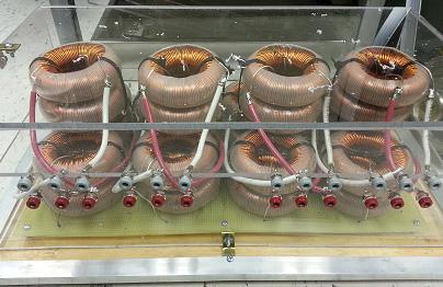
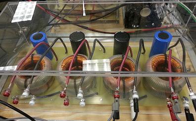
290 (a) (b) (c) (d) 265

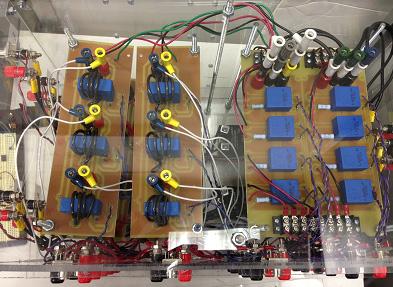
291 (e) (f) 266

292 (g) Figure 10.3 Hardware components developed for the implemented system: (a) uncontrolled rectifier, (b) AC filter, (c) DC filter, (d) controlled DC-DC boost converter, (e) AC measurement and protection box, (f) DC measurement and protection box and (g) load emulator. System Control and Operation Normally, the battery charger is operated in a current-control mode for charging and discharging the battery. In addition, the converter connected to the PV source is operated in a maximum power point tracking (MPPT) mode. Each of the boost converters is equipped with a local controller, moreover, a supervisor controller is used to monitor the operation of the various parts of the system, and act as a supervisory controller for the other local controllers. Several operational scenarios can be implemented using the developed testbed. Master-Slave (Communication-Based) Control Mode In this control technique, one of the DC-DC converters takes the charge of regulating the voltage on the DC bus, while the other converters operate in a current-control mode. The supervisory controller is responsible for selecting the converter that operates in the voltage-control mode, and sending current reference signals to the other converters. The 267

293 voltage-controlled converter in this case is analogous to the slack bus of an AC system, which regulates the frequency of the network and maintains the system power balance, however in this case it regulates the DC bus voltage. Moreover, the current-controlled converters are similar to the power-controlled buses in an AC network. Voltagecontrolled converters correspond to a voltage reference and yield a regulated DC voltage disregarding the load current and the input voltage, within a range. Current-controlled converters correspond to a reference current signal. A drawback of the master-slave control technique is its dependence on communication, which may decrease the reliability of the system. However, in modern smart grids, which are highly-based on reliable communication infrastructures, this architecture is more applicable since it can be integrated in wide are monitoring, control and protection systems and real-time management systems. Droop Control Mode Droop control is used to distribute a load between the source converters without any communication required among them. Each source converter s DC bus voltage is measured as a feedback signal, and then each of the source converters supply a portion of the power necessary to keep the system balanced, taking into consideration the losses of the DC power system. The droop characteristics of each controller can be designed such that the power sharing from each source is proportional to its rated capacity, or depending on its location, etc. The DC bus voltage decreases as the output current from the converter increase in order to provide a stable function. Heavy Load Mitigation Mode In order to mitigate the effect of these loads in the developed testbed, the converter in 268

294 the closest zone to the pulsed load is switched to the voltage-control mode, no matter what its initial stage is, in order to compensate for the voltage fluctuations expected. Moreover, the battery converter will be switched to a voltage-controlled mode so that it can supply as much energy as possible during the pulsed load, however, a saturation limit for the current drawn from the battery has to be pre-defined based on its power capacity. Several energy management algorithms can then be also implemented. Operational Results and Discussion In order to evaluate the performance of the developed DC distributed power system under different loading conditions and using different control architectures, several experiments were conducted. For control purposes, several dspace 1104 controller development systems were used as master and slave controllers. The switching frequency of the controlled converters used is 2 khz. In the first case study, the system is controlled such that the sharing from each zone is controlled. Each of the zones then corresponds automatically to any load changes and adjusts its output power to maintain the desired percent of demand it is controlled to follow. In this case, the four zones are controlled such that they equally share the demanded power as shown in figure Initially, a load of 1.9 kw is connected to the DC bus, it can be seen that each of the zones is sharing almost one fourth of the needed power. The load is then doubled to 3.8 kw, as can be seen, when the load is increased, the sharing from each zone increases as well, to maintain the load supplied, while maintaining the 25% sharing reference. This mode of operation is applicable when the generators of the system have close ratings and there is no preference on which generator should supply the load; if there is no consideration for the sharing, such as economic 269

295 dispatching or optimal load flow. Figure 10.5 shows the DC bus voltage in addition to the AC currents while running this experiment. It can be noticed that the DC voltage is stable; some voltage dip takes place when the load demand is increased then it settles down at its initial point. I 1 I 1 I 2 I 2 I 3 I 3 I 4 I 4 Figure 10.4 DC output currents from each of the four zones corresponding to a total load of 1.9 kw (initial), then a step change in the load to 3.8 kw (1.5 A/div, ms/div). V dc I a,b,c Figure 10.5 AC currents and DC voltage response to a total load of 1.9 kw (initial), then a step change in the load to 3.8 kw (Vdc: 300 V/div, 33.3 ms/div, Ia,b,c: 2 A/div, 33.3 ms/div). In case two, zones two, three and four were controlled through a PI current-controller. In this mode, a current reference value can be set. However, the boost converter 270

296 connected to one of the zones (zone 1 in this case) has to keep the voltage of the DC bus regulated. Hence, a voltage controller was used in zone 1. In order to examine this mode of operation, a set of current reference changes for zones 2, 3 and 4 were applied, I 4 is initially 2 A, then decreased to 1.6 A at zone 2. I 3 is initially 2 A, then decreased to 1.2 A at zone 3. I 4 is initially A, then decreased to 1.2 A at zone 4. Here, V dc that is controlled by zone 1 is set to 318 V. It can be seen that from figure 10.6 that zone 1, which is responsible for regulating the voltage is playing another essential role, which is to maintain the power balance in the network. When I 4, I 2 or I 3 decrease, I 1 increases to compensate and balance the power. Figure 10.7 shows the AC and DC voltages during the same experiment. It can be seen that the DC voltage is stable. Moreover, the AC voltages are not perfectly pure sinusoidal due to the fact that the system is relatively small; the generators ratings are not big compared to the demand. Hence, harmonics are of significant impact on the voltage wave shape. I 1 I 1 I 2 I 2 I 3 I 4 I 3 I 4 Figure 10.6 DC output currents response from each of the four zones corresponding to a set of step changes in the current reference (2 A/div, 0.2 s/div). 271

297 V dc V a,b,c Figure 10.7 AC voltages and DC voltage response to a set of load step changes (Vdc: 300 V/div, 33.3 ms/div, Va,b,c: 70 V/div, 33.3 ms/div). Protection Design and Equipment There are some technical challenges while designing a protection scheme for DC distribution systems, such as the fact that there is no zero crossing point for DC voltages and that fault interruptions must be done at high voltages, which is challenging and can reduce the life of the breakers. Moreover, the relatively low cable impedance of DC systems, along with the fast discharging of the DC link capacitor [205], may make the fault current rise to a very high value for a very short time in the range of <10 ms (down to less than 1ms). Hence, any breaker implemented on DC systems should have a reaction time that is in the range of 1 ms to 5 ms and even less. There is still research being conducted for developing better and more reliable ultra-fast circuit breakers in the order of µs reaction time. The protection coordination among the circuit breakers in DC systems is not well developed like in in the case of AC systems. The problem in DC systems is that the rise time of fault current is very high so it is practically difficult for the 272

298 breakers to differentiate the faults in different sections until there is an observable difference in any of the given parameters. The lack of standard DC voltage levels for DC distribution systems adds to the complexity of handling such systems. Another challenging issue related to the protection of DC systems is grounding. The grounding used on the AC side cannot be used directly for the DC side. A new ground should be created for the DC side separately. This way the DC and AC systems can be` separately protected from any ground faults. Case Study Description A protection system was designed to be implemented on the DC system that was presented earlier in this chapter. A schematic diagram of the system, from a protection point of view, is as shown in figure 10.8; it consists of four AC generators (two 13.8 kva plus two 10.4 kva) linked to a DC distribution system through an AC/DC conversion stage consisting of an uncontrolled rectifier in cascaded by a controlled boost converter. Moreover, the system also includes a battery storage system. AC Feeder For the AC feeder, being the bridge connecting the uncontrolled rectifiers to the generators, all the protection devices should be AC based. There are several protection schemes and devices already used in the industry for AC feeders. Some of these schemes, which are effective for the DC distributed power system application considered in this chapter, were implemented. Since the AC feeder is connected to the rectifiers directly, any fault might either influence the diodes of the rectifier or the inertia of the generators. Moreover, an AC feeder has some filtering characteristics since it can be modeled by an RL circuit at this length. Therefore, considering the limitations on the generator, filters 273

299 and the rectifier, the protection design and devices are selected. In this application, the under-frequency, over-frequency, under-voltage, over-voltage and over-current relay element schemes are designed. When any of the above relay scheme logic gets satisfied, a signal from the relay will be sent to open the AC breakers. The solid state breakers are used in this chapter, which has an operating voltage range of V. The transient peak overvoltage can go up to 1200 V with a maximum load current of 25 A. It has a good reaction time due to its maximum turn-on time and minimum turn-off time of ½ cycles. These specifications suit this application. (a) (b) Figure 10.8 A schematic diagram of the system under study; (a) layout of the system and faults locations, (b) snubber circuit. 274

300 The Converter The conversion from AC to DC is done here using two stages; an AC/DC uncontrolled rectifier stage cascaded by a DC/DC boost converter stage. As this combination is acting as a unit, any fault inside the converter is considered similar to a fault that occurs just outside the converter. The reason for this assumption is that separating the converter from the sources would obviously stop supplying power to the fault, which can be done by using the breakers right before and after the converter. Even though the converter is not included as one of the points of fault occurrence, its parameters, such as voltage and/or current, are very useful in controlling the fault situations and setting the critical limits for the protection devices. The diodes used in the uncontrolled rectifier have a specific current carrying capacity; beyond which they can be damaged. Therefore, using this parameter to set a limit would be one of the ideas to protect the converter. In this case, the overcurrent limit for the diodes is set to 3.08 p.u. DC Bus The DC bus is the place to which all the sources, loads and static storage elements are connected. The protection devices are placed right after the DC capacitor link of each sub-system. Disturbances on one of the sub-systems should not affect the power supplied to the load from any other sub-systems. Hence, using proper coordination schemes, the sub-section having the fault can only be isolated without interrupting the rest of the system. Another situation would be a disturbance right on the DC bus. In this case, there is an effect on the DC loads as well as the DC feeders connecting the supply and the converter to the DC bus. To protect the complete system, the breakers on the DC feeders have to 275

301 operate in order to separate all the sub-systems providing power to the DC bus. Moreover, the DC loads should be separated. Due to the very quick change in the DC current, practically it is difficult to identify and operate the breakers in that short time using the values of the current as relaying signals. Therefore, using the absolute value of the derivative of the current would help us detect the fault since the rise of the current will be faster than the actual current rise. This could help the circuit to react faster when the fault occurs. The interruption of this fault can be done using ultra-hybrid circuit breakers [206]. Using the voltage of the DC link would also be another way to interrupt the faults at the DC bus. Looking at the derivative of the converter current and the DC link voltage, the operation of the breakers are done in this study. The DC solid state breakers are used, which have a maximum turn-off time of 1 ms. They can be used in the voltage range of V at a maximum load current of 12 A. However, using molded case circuit breakers (MCCB) would also be another good option for this application. DC Loads Every sub-system has some local loads, just before the DC bus. There are two loads and a battery connected directly to the DC bus of the system. One load is the main highpriority load, while the other load and battery are of low priority. If there is any fault near the loads, using proper protection techniques and devices, the faulted areas or loads should only be separated to assure selectivity and maintain the operation for the rest of the system. In order to achieve this, separate ultra-fast DC fuses are installed near the loads. These DC fuses have a maximum turn-off time of 250µs, which is faster than any breaker in this system. The derivative of the DC current and the voltage across the DC link capacitor are also used to detect any faults that occur near the load location. So any 276

302 faults at the DC load will be disconnected with fuses and after the fault clearance they are manually changed. Grounding Grounding is mainly used in any system to protect it from any ground faults, moreover protective earthing is used to protect the personnel from electrical hazards. The AC generators are grounded through their star connections; this is used as the ground for the AC side. There are several grounding techniques for DC systems, such as isolated ground, high impedance grounding and low impedance grounding. However, the essential point to be considered is to have a separate grounding for AC and DC. To achieve this separate grounding scheme, an isolating transformer (star-star) [207] of 5 KVA on the AC feeder is used for each of the four subsystems. Now the question is which grounding scheme should be implemented on the DC side that well suits this application. Isolated ground would not be a good technique; firstly it is not safe to be implemented in a lab environment and secondly for any ground faults it would be difficult to detect and stabilize the system back to normal operation. Any of the two techniques, low impedance grounding and high impedance grounding can be used. The resistor value used for these grounding techniques should be a proper trade-off between ground currents and line to ground voltage [32]. In this application, the negative pole of the DC bus is grounded through a high resistance of 800 Ω as in IT-DC systems [208]. The ground current in normal conditions is observed to be around 3 ma, which is reasonably safe for the system. Fault Analysis and Coordination Scheme An exhaustive fault analysis is crucially needed in the process of developing an 277

303 efficient protection system. In this chapter, the focus is not just on analyzing the faults but also to explain some methods to interrupt those faults with suitable breakers, switches and fuses. Depending on the requirement, the protection devices are either used separately or in conjunction with other devices to protect the circuit. As the protection devices are set up at 4 different points in every sub-system, in addition to separate protection for the loads and battery, proper coordination among these protective devices has to be assured. This coordination of protection is dealt with while discussing each fault and the results collected for it. Initially, the fault analysis is done in PSCAD/EMTDC and the results are shown and explained. However, this same simulated environment is designed in the DC distributed architecture testbed providing a separate control center to observe all the measurements and control the protection equipment through dspace AC Side Faults The AC grid can face different faults, such as line to line fault, line to ground fault at the point shown in figure The sensitive components to be considered during the faults are the diodes of the converter and the DC link capacitor, with filters and cables being considered. In this application, since the system is small, any fault on AC side will have an insignificant impact on the DC loads. The current and voltage limits of the circuit are set based on the levels up to which the components can withstand. The overcurrent value is set to 1.23 p.u, overvoltage to 1.25 p.u, under-voltage to 0.75 p.u, over-frequency limit to 63 Hz and under-frequency to 57 Hz. Line-Line Fault A line to line fault at point 1 (FP1) on the AC side is shown in figure It can be 278

304 seen that the current levels on the AC side as well as the DC side rise for the faulted phases, while the voltages drop down. As observed from figure 10.9(a), the AC current is crossing the overcurrent limit of 1.23 p.u after 3.5 ms, and the signal started from zero (fault being between phases A and B). While the line to ground voltage (peak) of phases A and B shown in figure 10.9(b) drops down below the under-voltage limit of 0.75 p.u and this happens after 8.0 ms, the signal started from zero. Moreover, what can be also observed in this scenario is that the phase angle of current between phases A and B became after the fault, while the current in the un-faulted phase becomes almost zero. This can be used as an effective detection parameter if synchronized measurements are available. Moreover, if the response of this fault on the DC side is observed, the bus voltage and the DC bus current stay within the safe limits because of the filter capacitance and inductance present after the un-controlled rectifier. Next, the aim would be to clear this fault in the shortest possible time because the AC current crosses the current limit of the circuit, which is 1.23 p.u. The AC solid state relays detect the fault, to operate the breakers in 8.3 ms to clear the fault. The frequency remains the same after the fault, but the under-frequency and over-frequency limits are set in any emergency situations. With the operation of the AC breakers, the generator is separated from the circuit and the diode current is within limits. However, the DC breakers must be operated to isolate this sub-system. The relays used are accompanied with a reclosing scheme, so that after the fault clearance, the breakers reclose to continue the normal operation of the circuit. After 180 ms from the fault occurrence, the breakers are reclosed as observed from the graph considering the fault is cleared before this reclose. Due to this reclosing action, the DC current can rise to a high level. Therefore, in order to limit this 279

305 high current, a DC RL- snubber circuit is used. This snubber circuit was designed, Fig 10.8(b), to control the arc during the reclosing phenomena. When the breaker is open, the IGBT blocks the current flow through it by using the relay signal from breaker. This relay signal first opens the IGBT and then the breaker. While reclosing, before the breaker closes, the IGBT closes in that very short time gap. So the arc goes through the snubber and reduces its impact on the main circuit. 3 2 Current [P.U.] Time [s] 1 (a) 0.5 Voltage [P.U.] Time [s] (b) Figure 10.9 Line to Line fault at FP1; (a) current in phases A and B 180 apart and crossing limit of 1.23 p.u, (b) line to ground voltage going less than undervoltage limit of 0.75 p.u. Line-Ground Fault At the same point FP1 in figure 10.8, the possibility of a line to ground fault is 280

306 discussed. As observed from figure 10.10(a) the phase voltage of phase A became zero after the fault and the current value in that phase observed from figure 10.10(b) rose to a high value of about 3.0 p.u. As the overcurrent limit is set at 1.23 p.u, the relay operates as the current value crosses this limit. Having a good response time of 8.3 ms for the breakers, it is flexible to protect the circuit and isolate it. Inspecting the effect of the fault on the DC side, no significant effect can be noticed. The snubber design assures a reduction in the effect of the arc. Coordination on the AC side To operate the breakers in a proper coordination for these faults, some priority setting has to be kept in mind. Looking at the results of figures 10.9 and the AC breaker should be operated first to isolate the AC supply followed by the DC breakers to protect the sub-system. However, the DC breakers are operated from the signal generated by the AC relays. As for the Line-Ground fault, the same coordination scheme used for the line to line fault and the line to ground fault is operated and cleared. DC Side Faults DC grid faults are discussed in this section analyzing each fault separately while explaining the possible relaying and protection coordination. The relays are operated based on over-current, over-voltage and under-voltage limits settings for the circuit. There are two sections involved in this case; one with the DC bus connecting each of the sub-systems and the other one would be the loads and the battery connected to the bus. Proper coordination is required to differentiate faults at the crucial points of the system. The over-current limit is set at 1.23 p.u, under-voltage and over-voltage limits at p.u and p.u, respectively. 281

307 3 2 Current [P.U.] Time [s] 1 (a) 0.5 Voltage [P.U.] Time [s] (b) Figure Line to Ground fault at FP1; (a) current crossing the limit of 1.23 p.u, (b) line to ground voltage going less than undervoltage of 0.75 p.u. Fault at the DC Bus (FP2) The possible faults that might occur on the DC side are at FP2, FP3, and FP4 of the system. These points are dealt with separately then the coordination scheme to differentiate these faults is analyzed. Firstly, considering a fault at FP2, which is the DC bus location, the results are depicted in figure At the instant of fault, there is a sudden change in the DC current due to the fast capacitor discharge. As explained earlier in this chapter, using the derivative would help us quickly detect the fault and consequently use ultra-hybrid circuit breakers to interrupt the fault. The limit for the 282

308 derivative of DC current is set at 1.23 p.u/ms. As can be observed in figure 10.11(a) the derivative of the DC current reaches the limit of 1.23 p.u/ms in less than 500 µs. Therefore, using an ultra-hybrid circuit breaker, a 300 µs interruption time can be reached [206], which is quite sufficient for this application. Furthermore, the derivative of the voltage at the DC link, figure 10.11(b) drops down to 0.85 p.u, which crosses the undervoltage limit. The relay operation is done using the derivative of the DC current along with the DC link under-voltage in combination. The effect of this fault is observed on the AC current and voltages which are interrupted by the AC breakers. The load voltage drops down very low due to the fault on the bus, which affects all the sources connecting the load. Fault at the DC load (FP3) FP3 is the point of concern when it comes to the load because it is considered as highpriority load. This fault has an influence on the complete system, and has more influence on the load. The effect of this fault is very similar to FP2 but there will be difference at the time scale of ms between the two of them. This is discussed during coordination. The detection of this fault is done using the derivative of the DC current along with the DC link voltage. It is observed that the separation of load is done very fast before the AC and DC breakers could receive the relay signal. Fault at the battery can be interpreted the same way as the loads, but with different protection limits which can be much higher than those for the loads. Coordination Scheme on the DC Side The most important operation of the complete protection system lies in the 283

309 coordination of breakers. For any specific fault, the breaker that is responsible and required to clear the fault should be operated. A normal breaker cannot differentiate faults at different points in the system. It just opens and closes based on the relay signals. So the relays are responsible to operate the breakers in a coordinated scheme DC current derivative [P.U/ms] Time [s] (a) 2 DC bus voltage [P.U] Time [s] (b) Figure Pole to Pole fault at point FP2; (a) derivative of the DC current, (b) DC bus voltage. In this application, the fault points to be differentiated are (FP2, FP3) and (FP2, FP4). The first task would be to pick up the parameter that best differentiates the fault and the second task would be to select the appropriate breaker to open. From figure (a), it is clear that the derivative of the DC current due to FP2 has more slope than the derivative of the DC current due to FP3. Moreover, the DC bus voltage reaches zero, 284

310 figure (b) due to FP2 faster than that due to FP3, where the derivative of the DC link voltage can depict the difference. These two parameters can differentiate the faults FP2 and FP3. The next situation would be between FP2 and FP4. For this case, the ultrafast fuses installed at the DC load are the primary reason to distinguish the faults. For any fault at FP4, the load branch, being the high-priority load separates itself very fast so that there will be no fault in the system to open the DC breakers and AC breakers. The remaining loads open even faster than the high-priority load as the ultra-fast fuses have <250µs reaction time. Current derivative [P.U/ms] FP4 FP2 500 DC link voltage derivative [P.U/ms] Time [s] (a) FP4 FP Time [s] (b) Figure Coordination between the faults at FP2 and FP4; (a) derivative of the DC current, (b) derivative of the bus voltage. 285

311 Distribution Architectures Implementation The developed testbed has a reconfiguration capability, which enables us to compare the performance of the various distribution architectures in a power system. As an example, the four distribution architectures that may be used on a shipboard power system will be compared. These architectures are the Radial AC, Medium Voltage DC and Zonal DC distribution systems and they will all be implemented on the developed power system testbed. Figure shows a general overview of the testbed and its reconfiguration capability. The system consists of 5 busses; four of which are AC buses and bus 5 represents the microgird. Each of the AC busses consists of a prime movergenerator set cascaded by two possible paths for the power entering the bus giving two options. If Sac is ON and Sdc is OFF, the power will flow in an AC form to the bus. However, if Sdc is ON and Sac is OFF the power will flow to the bus through an AC/DC rectifier yielding DC power. This flexibility of supplying the system with AC or DC power allows the reconfiguration of the system to test different architectures. The DC microgrid involves fuel cell generation, battery storage and super capacitors. Sac and Sdc do the same role here as explained earlier. Switches designated S1:S8 give more flexibility and reconfiguration capability to the system. AC Radial Distribution In this architecture, the power flows in a radial manner. Every bus is just connected to the bus/buses physically existing around it. This will be implemented on the testbed by switching S1, S3, S6, S8 and Sac ON; and switching S2, S4, S5, S7 and Sdc OFF. Figure shows the power flow in the testbed with the radial architecture implemented. 286

312 Figure The developed reconfigurable testbed. Figure Radial AC distribution. Medium Voltage DC Distribution Medium voltage DC power distribution systems are being considered for future naval warships. There are several design considerations attached to them. In this case, all the generators will be sharing DC power. This will be implemented on the testbed by switching S1:S8 and Sdc ON; and switching Sac OFF. Figure shows the power flow in the testbed with the medium voltage DC distribution architecture implemented. 287