Comparison of Macrotexture Measurement Methods. Master s Thesis. Presented in Partial Fulfillment of the Requirements for the Degree Master of Science

Transcription

1 Comparison of Macrotexture Measurement Methods Master s Thesis Presented in Partial Fulfillment of the Requirements for the Degree Master of Science By Nicholas R. Fisco Graduate Program in Civil Engineering The Ohio State University 2009 Thesis Committee Halil Sezen, Advisor Hojjat Adeli Shive Chaturvedi

2 Copyright by Nicholas Robert Fisco 2009

3 Abstract This study investigates and compares mean profile depth (MPD) measurements from three laser-based macrotexture measuring devices, namely a Dynatest laser profiler, a Circular Texture Meter, and an Ames Laser Texture Scanner, to mean texture depth (MTD) results from volumetric sand patch tests. In addition, the effects of speed and material type on the MPD results for the profiler are researched. The effect of macrotexture on surface friction is also investigated using a Dynamic Friction Tester. The study uses sand patch test data obtained from field testing at three sites, each with a variety of pavement types, and laboratory testing on various types of Hot Mix Asphalt (HMA) and Portland cement concrete samples of varying finish, as well as other common, manufactured, textured samples. Analysis of the data shows that the MPD obtained from the Ames Laser Texture Scanner has the highest correlation to the MTD measurements determined using the sand patch test. It is also determined that the MPD values taken by the laser profiler decreased as the speed at which the sample was traveling increased. A new correlation for predicting MTD from laser profiler MPD is developed through laboratory testing. Additionally, it is found that material type had an effect on the laser MPD values. ii

4 Acknowledgements The authors would like to thank the following people and entities for their help with this study: Dr. Halil Sezen Brian Schleppi, ODOT Roger Green, ODOT Daniel Radanovich, ODOT Jay Hunter, OSU Donald and Patricia Fisco Michael Fisco, American Corrugated Joseph Danatzko The Ohio State University Center for Automotive Research (CAR) Mark Leichty and Ames Engineering Kevin Williams, Burns, Cooley, Dennis FHWA Randall Milton, Dynatest Lutron iii

5 Vita May 2003 Gallia Academy High School 2007 B.S. Civil Engineering, The Ohio State University 2005 to 2006 Intern, Ohio Department of Transportation 2006 to 2007 Intern, Burgess and Niple 2007 Field Technician Intern, BBCM 2008 to 2009 Graduate Research Assistant, Department of Civil and Environmental Engineering and Geodetic Science, The Ohio State University 2009 French Fellowship Recipient Major Field: Civil Engineering Field of Study iv

6 TABLE OF CONTENTS LIST OF FIGURES... IX LIST OF TABLES... XVII CHAPTER 1 INTRODUCTION AND OBJECTIVES... 1 SECTION 1.1 INTRODUCTION... 1 SECTION 1.2 OBJECTIVES... 4 SECTION 1.3 ORGANIZATION... 6 CHAPTER 2 LITERATURE REVIEW... 7 SECTION 2.1 SURFACE TEXTURE MEASUREMENTS... 7 SECTION 2.2 DIGITAL IMAGERY SECTION 2.3 PAVEMENT FRICTION CHARACTERISTICS SECTION 2.4 ASTM STANDARDS CHAPTER 3 BACKGROUND INFORMATION AND ODOT FIELD TESTING SECTION 3.1 INTRODUCTION SECTION 3.2 FIELD TESTING SECTION 3.3 IMPLEMENTATION OF FIELD TESTING RESULTS AND RESEARCH IMPETUS CHAPTER 4 SAMPLE PROPERTIES SECTION 4.1 INTRODUCTION SECTION 4.2 ASPHALT SAMPLES SECTION 4.3 CONCRETE SAMPLES SECTION 4.4 OTHER SAMPLES v

7 CHAPTER 5 COMPUTED TOMOGRAPHY SCANNING SECTION 5.1 INTRODUCTION SECTION 4.2 CT SCANNING OF SAMPLES SECTION 4.3 DEFICIENCIES AND FUTURE OF CT SCANNING CHAPTER 6 LABORATORY SAND PATCH TESTING OF SAMPLES SECTION 6.1 INTRODUCTION SECTION 6.2 TESTING PROCEDURE SECTION 6.3 SAND PATCH TEST RESULTS CHAPTER 7 DYNATEST LASER PROFILER LABORATORY TESTING OF SAMPLES SECTION 7.1 INTRODUCTION SECTION 7.2 TEST SETUP SECTION 7.3 TESTING METHOD SECTION 7.4 EVALUATION OF TEST RESULTS Subsection Material Sensitivity Subsection Speed Sensitivity CHAPTER 8 AMES LASER TEXTURE SCANNER TESTING OF LABORATORY SAMPLES SECTION 8.1 SCANNER DETAILS SECTION 8.2 TESTING PROCEDURE SECTION 8.3 EVALUATION OF RESULTS CHAPTER 9 CT METER TESTING OF LABORATORY SAMPLES SECTION 9.1 CT METER DETAILS SECTION 9.2 TESTING PROCEDURE SECTION 9.3 RESULTS OF CT METER TESTS vi

8 CHAPTER 10 DYNAMIC FRICTION TESTS SECTION 10.1 DYNAMIC FRICTION TESTER DETAILS SECTION 10.2 TESTING PROCEDURE SECTION 10.3 DYNAMIC FRICTION TEST RESULTS SECTION 10.4 INTERNATIONAL FRICTION INDEX CALCULATIONS CHAPTER 11 COMPARISON OF SURFACE MACROTEXTURE METHODS SECTION 11.1 TWO-DIMENSIONAL VERSUS THREE-DIMENSIONAL METHODS SECTION 11.2 COMPARISON OF MTD AND ETD VALUES SECTION 11.3 COMPARISON OF METHODS USING STATISTICAL ANALYSIS SECTION 11.4 COMPARISON OF SAND PATCH MTD AND MPD USING GRAPHICAL APPROACH Subsection Comparison Using Ames Scanner MPD Subsection Comparison Using CT Meter MPD Subsection Comparison Using Dynatest Laser Profiler MPD SECTION 11.5 COMPARISON OF ETD AND MPD USING GRAPHICAL APPROACH SECTION 11.6 COMPARISON OF ETD VALUES CHAPTER 12 CONCLUSIONS AND RECOMMENDATIONS SECTION 12.1 SUMMARY OF WORK SECTION 12.2 CONCLUSIONS SECTION 12.3 LIMITATIONS AND SOURCE OF ERROR SECTION 12.4 RECOMMENDATIONS SECTION 12.5 IMPLEMENTATION BIBLIOGRAPHY APPENDIX A SAMPLE IMAGES APPENDIX B CT SCAN SUPPLEMENTAL FIGURES APPENDIX C SAND PATCH DATA SHEETS vii

9 APPENDIX D AMES SCANNER RENDERINGS VS. CT SCAN IMAGES APPENDIX E CT METER PROFILES APPENDIX F DFT FRICTION COEFFICIENT GRAPHS APPENDIX G SUPPLEMENTAL GRAPHS, TABLES, AND METRIC EQUIVALENTS APPENDIX H SUPPLEMENTAL PHOTOS viii

10 LIST OF FIGURES Figure 3.1 Sand Patch Tests Carried Out on Smooth AC Section of ODOT Certification Course 26 Figure 3.2 Sand Patch Test Carried Out on 1984 AC Section of Goodyear Test Track 26 Figure 3.3 Tined Concrete at ODOT Certification Course 26 Figure 3.4 Sand Patch Test Carried Out on Ground Concrete Section of ODOT Certification Course 27 Figure 4.1 SMA Asphalt Sample and Surface Texture 34 Figure 4.2 Burlap Drag PCC #2 Sample and Surface Texture 38 Figure 4.3 Turf Drag PCC #2 Sample and Surface Texture 38 Figure 4.4 Rubber Stepping Stone Sample and Surface Texture 41 Figure 5.1 SOMATOM Sensation Cardiac CT Scanner with Asphalt Specimens 45 Figure 5.2 Exposed Aggregate PCC, CT Scan Rendering 46 Figure 5.3 Exposed Aggregate PCC Two-Dimensional CT Scan Slice 46 Figure 5.4 Exposed Aggregate PCC CT Scan Rendering 47 Figure 5.5 Open Grade Asphalt Concrete CT Scan Rendering 47 Figure 5.6 Open Grade Asphalt Concrete Two-Dimensional CT Scan Slice 48 Figure 5.7 Open Grade Asphalt Concrete CT Scan Rendering 48 Figure 6.1 PCC Exposed Aggregate Sand Patch Tests 52 Figure 7.1 Test Apparatus 57 Figure 7.2 Test Setup with ODOT Profiler Van on Ramps 58 Figure 7.3 Correction Factor versus Speed 70 Figure 8.1 Ames Laser Texture Scanner Top and Bottom Views 71 Figure 8.2 Scanner Test Positions 74 Figure 8.3 Three Dimensional Surface Rendering From Ames Scanner Exposed Aggregate PCC 78 Figure 8.4 Exposed Aggregate PCC CT Scan Rendering 78 Figure 9.1 CT Meter Bottom View 80 Figure 9.2 CT Meter Top View 80 Figure 9.3 Test Rig Bottom Platform 81 Figure 9.4 CT Test Rig Side View 81 ix

11 Figure 9.5 CT Meter and Test Rig Side View 82 Figure 9.6 Radial Tine Surface Profile 84 Figure 9.7 Broom Drag 2 Surface Profile 85 Figure 9.8 Exposed Aggregate 1 Surface Profile 85 Figure 10.1 DFT Top View 87 Figure 10.2 DFT Bottom View 87 Figure 10.3 DFT Worn and Unworn Friction Pads 87 Figure 10.4 DFT Setup 87 Figure 10.5 DFT and Rig Side View 88 Figure 10.6 DFT Rig Side View 89 Figure 10.7 Measure Friction Coefficient versus Speed for Exposed Aggregate PCC 2 92 Figure 10.8 Measure Friction Coefficient versus Speed for Smooth PCC 1 92 Figure 10.9 CT Meter ETD versus Friction Coefficients at Varying Speeds 93 Figure CT Meter ETD versus International Friction Index 97 Figure F60 versus DFT Measurements at 49.7 mph (60 km/h) 98 Figure F60 versus DFT Measurements at 49.7 mph (60 km/h) No Porous Samples 99 Figure 11.1 Laser Profiler Path Position on Longitudinal Tines 101 Figure 11.2 Laser Profiler Path Position on Transverse Tines 102 Figure 11.3 Sand Patch MTD versus Ames MPD with Outliers 115 Figure 11.4 Linear Relation and Coefficients of Correlation for Ames with No Outliers 116 Figure 11.5 Linear Relation and Coefficients of Correlation for CT Meter with Outliers 117 Figure 11.6 Linear Relation and Coefficients of Correlation for CT Meter No Outliers 118 Figure 11.7 Linear Relation and Coefficients of Correlation for Dynatest Profiler at 25 mph 119 Figure 11.8 Linear Relation and Coefficients of Correlation for Dynatest Profiler at 35 mph 120 Figure 11.9 Linear Relation and Coefficients of Correlation for Dynatest Profiler at 45 mph 120 Figure Linear Relation and Coefficients of Correlation for Dynatest Profiler at 55 mph 121 Figure Overall Linear Relation and Coefficient of Correlation for Dynatest Profiler 123 Figure Sand Patch MTD versus ETD from Sand Patch Relations in Table Figure CT Meter ETD versus Dynatest ETD at 11 in. Diameter using ASTM Relations 132 Figure Ames ETD versus ETD at All Diameters using ASTM Relations 134 Figure 12.1 Summary of Areas or Path Tested on Each Sample 136 Figure 12.2 Procedures and Results 137 Figure A.1 Alpine Panel 149 Figure A.2 Broom Drag PCC #1 149 x

12 Figure A.3 Broom Drag PCC #2 149 Figure A.4 Burlap Drag PCC #1 150 Figure A.5 Burlap Drag PCC #2 150 Figure A.6 Burlap Layover PCC #1 150 Figure A.7 Cheyenne Panel 151 Figure A.8 Dense Grade Asphalt Concrete 151 Figure A.9 Exposed Aggregate PCC #1 151 Figure A.10 Exposed Aggregate PCC #2 152 Figure A.11 Open (Coarse) Grade Asphalt Concrete #1 152 Figure A.12 Open (Coarse) Grade Asphalt Concrete #2 152 Figure A.13 Granite Stepping Stone 153 Figure A.14 Rubber Stepping Stone 153 Figure A.15 Stone Matrix Asphalt (SMA) Concrete #1 153 Figure A.16 Stone Matrix Asphalt (SMA) Concrete #2 154 Figure A.17 Smooth PCC #1 154 Figure A.18 Smooth PCC #2 154 Figure A Grit Sandpaper 155 Figure A Grit Sandpaper 155 Figure A Grit Sandpaper 155 Figure A.22 Radial Tine #1 156 Figure A.23 Radial Tine #2 156 Figure A.24 Tivoli Ceiling Tile 156 Figure A.25 Turf Drag PCC #1 157 Figure A.26 Turf Drag PCC #2 157 Figure B.1.1 Turf Drag PCC CT Scan Renderings 159 Figure B.1.2 Turf Drag PCC 2-D CT Scan Slice 159 Figure B.1.3 Turf Drag PCC 2-D CT Scan Slice Enhanced 160 Figure B.1.4 Turf Drag PCC CT Scan Rendering 160 Figure B.2.1 Dense Grade Asphalt Concrete CT Scan Renderings 161 Figure B.2.2 Dense Grade Asphalt Concrete 2-D CT Scan Slice 161 Figure B.2.3 Dense Grade Asphalt Concrete 2-D CT Scan Slice Enhanced 162 Figure B.2.4 Dense Grade Asphalt Concrete CT Scan Rendering 162 Figure B.3.1 Open Grade Asphalt Concrete CT Scan Renderings 163 Figure B.3.2 Open Grade Asphalt Concrete 2-D CT Scan Slice 163 xi

13 Figure B.3.3 Open Grade Asphalt Concrete 2-D CT Scan Slice Enhanced 164 Figure B.3.4 Open Grade Asphalt Concrete CT Scan Rendering 164 Figure D.1 Three Dimensional Surface Rendering From Ames Scanner Dense Grade Asphalt Top and Side Views 172 Figure D.2 Three Dimensional Surface Rendering From CT Scan Dense Grade Asphalt Top and Side Views 172 Figure D.3 Three Dimensional Surface Rendering From Ames Scanner Turf Drag PCC Top and Side Views 173 Figure D.4 Three Dimensional Surface Rendering From CT Scan Turf Drag PCC Top and Side Views 173 Figure D.5 Three Dimensional Surface Rendering From Ames Scanner Open Grade Asphalt Top and Side Views 174 Figure D.6 Three Dimensional Surface Rendering From Ct Scan Open Grade Asphalt Top and Side Views 174 Figure E.1 50 Grit Sandpaper Profile 176 Figure E.2 60 Grit Sandpaper Profile 176 Figure E.3 60 Grit Sandpaper Profile 176 Figure E.4 Alpine Panel Profile 176 Figure E.5 Broom 1 PCC Profile 177 Figure E.6 Broom 2 PCC Profile 177 Figure E.7 Burlap Drag 1 PCC Profile 177 Figure E.8 Burlap Drag 1 PCC Profile 177 Figure E.9 Burlap Layover PCC Profile 178 Figure E.10 Dense Grade Asphalt Profile 178 Figure E.11 Exposed Aggregate 1 PCC Profile 178 Figure E.12 Exposed Aggregate 2 PCC Profile 179 Figure E.13 Open Grade Asphalt 1 Profile 179 Figure E.14 Open Grade Asphalt 2 Profile 180 Figure E.15 Radial Tine 1 Profile 180 Figure E.16 Radial Tine 2 Profile 180 Figure E.17 Rough Granite Profile 181 Figure E.18 Rubber Stepping Stone Profile 181 Figure E.19 SMA 1 Profile 181 Figure E.20 SMA 2 Profile 182 xii

14 Figure E.21 Smooth 1 PCC Profile 182 Figure E. 22 Smooth 2 PCC Profile 182 Figure E.23 Smooth Granite Profile 182 Figure E.24 Tivoli Tile Profile 183 Figure E.25 Turf Drag 1 PCC Profile 183 Figure E.26 Turf Drag 2 PCC Profile 183 Figure F.1 Broom 1 PCC Graph 185 Figure F.2 Broom 2 PCC Graph 185 Figure F.3 Burlap Drag 1 PCC Graph 185 Figure F.4 Burlap Drag 2 PCC Graph 186 Figure F.5 Burlap Layover PCC Graph 186 Figure F.6 Dense Grade Asphalt Graph 186 Figure F.7 Exposed Aggregate 1 PCC Graph 187 Figure F.8 Exposed Aggregate 2 PCC Graph 187 Figure F.9 Open Grade Asphalt 1 Graph 187 Figure F.10 Open Grade Asphalt 2 Graph 188 Figure F.11 Rubber Stepping Stone Graph 188 Figure F.12 SMA 1 Graph 188 Figure F.13 SMA 2 Graph 189 Figure F.14 Smooth 1 PCC Graph 189 Figure F.15 Smooth 2 PCC Graph 189 Figure F.16 Radial Tine 1 PCC Graph 190 Figure F.17 Radial Tine 2 PCC Graph 190 Figure F.18 Turf Drag 1 PCC Graph 190 Figure F.19 Turf Drag 2 PCC Graph 191 Figure G.1 (10.8M) CT Meter ETD versus Friction Coefficients at Varying Speeds 197 Figure G.2 Sand Patch MTD versus Ames MPD with Outliers 198 Figure G.3 Linear Relation and Coefficients of Correlation for Ames with No Outliers 198 Figure G.4 Linear Relations and Coefficients of Correlation for Dynatest Profiler at 40 km/h 199 Figure G.5 Linear Relations and Coefficients of Correlation for Dynatest Profiler at 56 km/h 199 Figure G.6 Linear Relations and Coefficients of Correlation for Dynatest Profiler at 72 km/h 200 Figure G.7 Linear Relations and Coefficients of Correlation for Dynatest Profiler at 89 km/h 200 Figure G.8 Overall Linear Relation and Coefficient of Correlation for Dynatest Profiler 201 Figure G.9 Ames ETD versus CT Meter MPD Correlation with Outliers 204 xiii

15 Figure G.9M Ames ETD versus CT Meter MPD Correlation with Outliers 204 Figure G.10 Ames ETD versus CT Meter MPD Correlation without Outliers 205 Figure G.10M Ames ETD versus CT Meter MPD Correlation without Outliers 205 Figure G.11 Ames ETD versus Dynatest MPD at 25 mph Correlation 206 Figure G.11M Ames ETD versus Dynatest MPD at 40 km/h Correlation 206 Figure G.12 Ames ETD versus Dynatest MPD at 35 mph Correlation 207 Figure G.12M Ames ETD versus Dynatest MPD at 56 km/h Correlation 207 Figure G.13 Ames ETD versus Dynatest MPD at 45 mph Correlation 208 Figure G.13M Ames ETD versus Dynatest MPD at 72 km/h Correlation 208 Figure G.14 Ames ETD versus Dynatest MPD at 55 mph Correlation 209 Figure G.14M Ames ETD versus Dynatest MPD at 89 km/h Correlation 209 Figure G.15 CT Meter ETD versus Ames MPD Correlation with Outliers 210 Figure G.15M CT Meter ETD versus Ames MPD Correlation with Outliers 210 Figure G.16 CT Meter ETD versus Ames MPD Correlation without Outliers 211 Figure G.16M CT Meter ETD versus Ames MPD Correlation without Outliers 211 Figure G.17 CT Meter ETD versus Dynatest MPD at 25 mph Correlation with Outliers 212 Figure G.17M CT Meter ETD versus Dynatest MPD at 40 km/h Correlation with Outliers 212 Figure G.18 CT Meter ETD versus Dynatest MPD at 25 mph Correlation without Outliers 213 Figure G.18M CT Meter ETD versus Dynatest MPD at 40 km/h Correlation without Outliers 213 Figure G.19 CT Meter ETD versus Dynatest MPD at 35 mph Correlation with Outliers 214 Figure G.19M CT Meter ETD versus Dynatest MPD at 56 km/h Correlation with Outliers 214 Figure G.20 CT Meter ETD versus Dynatest MPD at 35 mph Correlation without Outliers 215 Figure G.20M CT Meter ETD versus Dynatest MPD at 56 km/h Correlation without Outliers 215 Figure G.21 CT Meter ETD versus Dynatest MPD at 45 mph Correlation with Outliers 216 Figure G.21M CT Meter ETD versus Dynatest MPD at 72 km/h Correlation with Outliers 216 Figure G.22 CT Meter ETD versus Dynatest MPD at 45 mph Correlation without Outliers 217 Figure G.22M CT Meter ETD versus Dynatest MPD at 72 km/h Correlation without Outliers 217 Figure G.23 CT Meter ETD versus Dynatest MPD at 55 mph Correlation with Outliers 218 Figure G.23M CT Meter ETD versus Dynatest MPD at 89 km/h Correlation with Outliers 218 Figure G.24 CT Meter ETD versus Dynatest MPD at 55 mph Correlation without Outliers 219 Figure G.24M CT Meter ETD versus Dynatest MPD at 89 km/h Correlation without Outliers 219 Figure G.25 Dynatest ETD versus Ames MPD Correlations 220 Figure G.25M Dynatest ETD versus Ames MPD Correlations 220 Figure G.26 Dynatest ETD versus CT Meter MPD Correlations with Outliers 221 xiv

16 Figure G.26M Dynatest ETD versus CT Meter MPD Correlations with Outliers 221 Figure G.27 Dynatest ETD versus CT Meter MPD Correlations without Outliers 222 Figure G.27M Dynatest ETD versus CT Meter MPD Correlations without Outliers 222 Figure G.28 Dynatest ETD at 25 mph versus Dynatest MPD at 35 mph Correlation 223 Figure G.28M Dynatest ETD at 40 km/h versus Dynatest MPD at 56 km/h Correlation 223 Figure G.29 Dynatest ETD at 25 mph versus Dynatest MPD at 45 mph Correlation 224 Figure G.29M Dynatest ETD at 40 km/h versus Dynatest MPD at 72 km/h Correlation 224 Figure G.30 Dynatest ETD at 25 mph versus Dynatest MPD at 55 mph Correlations 225 Figure G.30M Dynatest ETD at 40 km/h versus Dynatest MPD at 89 km/h Correlations 225 Figure G.31 Dynatest ETD at 35 mph versus Dynatest MPD at 25 mph Correlations 226 Figure G.31M Dynatest ETD at 56 km/h versus Dynatest MPD at 40 km/h Correlations 226 Figure G.32 Dynatest ETD at 35 mph versus Dynatest MPD at 45 mph Correlations 227 Figure G.32M Dynatest ETD at 56 km/h versus Dynatest MPD at 72 km/h Correlations 227 Figure G.33 Dynatest ETD at 35 mph versus Dynatest MPD at 55 mph Correlations 228 Figure G.33M Dynatest ETD at 56 km/h versus Dynatest MPD at 89 km/h Correlations 228 Figure G.34 Dynatest ETD at 45 mph versus Dynatest MPD at 25 mph Correlations 229 Figure G.34M Dynatest ETD at 72 km/h versus Dynatest MPD at 40 km/h Correlations 229 Figure G.35 Dynatest ETD at 45 mph versus Dynatest MPD at 35 mph Correlations 230 Figure G.35M Dynatest ETD at 72 km/h versus Dynatest MPD at 56 km/h Correlations 230 Figure G.36 Dynatest ETD at 45 mph versus Dynatest MPD at 55 mph Correlations 231 Figure G.36M Dynatest ETD at 72 km/h versus Dynatest MPD at 89 km/h Correlations 231 Figure G.37 Dynatest ETD at 55 mph versus Dynatest MPD at 25 mph Correlations 232 Figure G.37M Dynatest ETD at 89 km/h versus Dynatest MPD at 40 km/h Correlations 232 Figure G.38 Dynatest ETD at 55 mph versus Dynatest MPD at 35 mph Correlations 233 Figure G.38M Dynatest ETD at 89 km/h versus Dynatest MPD at 56 km/h Correlations 233 Figure G.39 Dynatest ETD at 55 mph versus Dynatest MPD at 45 mph Correlations 234 Figure G.39M Dynatest ETD at 89 km/h versus Dynatest MPD at 72 km/h Correlations 234 Figure G.40 Sand Path MTD versus ETD from Ames Relations 235 Figure G.40M Sand Path MTD versus ETD from Ames Relations 235 Figure G.41 Sand Path MTD versus ETD from CT Meter Relations 236 Figure G.41M Sand Path MTD versus ETD from CT Meter Relations 236 Figure G.42 Sand Path MTD versus ETD from Dynatest at 25 mph Relations 237 Figure G.42M Sand Path MTD versus ETD from Dynatest at 40 km/h Relations 237 Figure G.43 Sand Path MTD versus ETD from Dynatest at 35 mph Relations 238 xv

17 Figure G.43M Sand Path MTD versus ETD from Dynatest at 56 km/h Relations 239 Figure G.44 Sand Path MTD versus ETD from Dynatest at 45 mph Relations 239 Figure G.44M Sand Path MTD versus ETD from Dynatest at 72 km/h Relations 240 Figure G.45 Sand Path MTD versus ETD from Dynatest at 55 mph Relations 240 Figure G.45M Sand Path MTD versus ETD from Dynatest at 89 km/h Relations 241 Figure G.46 (11.10M) Sand Path MTD versus ETD from Sand Patch Relations 241 Figure F.1 Concrete Molds 243 Figure F.2 Mixing of Concrete Used for Samples 243 Figure F.3 Broom Drag PCC Sample in Mold With Broom Used for Finishing 243 Figure F.4 Turf Drag PCC Sample in Mold With Turf Used for Finishing 244 Figure F.5 Exposed Aggregate PCC Sample in Mold After Top Mortar Removal With Water 244 Figure F.6 Asphalt Samples After Fabrication at Kokosing Materials Laboratory in Mansfield, OH 244 Figure F.7 14-in. Metal Ring Used for Fabricating Asphalt Samples Metal Ring Cut From 14-in. Diameter Metal Drum 245 Figure F.8 SMA Asphalt Sample With Restraining Collar Made From Hose Clamps Riveted to Sheet Metal 245 Figure F.9 Wheel Path View of Testing Apparatus 246 Figure F.10 Top Down View of Test Apparatus 246 Figure F.11 Ames Scanner Laser Dot on Samples 246 xvi

18 TABLES Table 3.1 Site Details for ODOT Field Testing 25 Table 3.2 Sand Patch Test Results for the Smooth AC Pavement Section of ODOT Certification Course 27 Table 3.3 Comparison of All Field Sand Patch Samples 28 Table 3.4 Results of Dynatest Profiler for Smooth AC Section of ODOT Certification Course 29 Table 3.5 Comparison of Average MTD and ETD Values for Each Pavement Type 30 Table 4.1 Stone Matrix Asphalt Mix Design 34 Table 4.2 Coarse Grade Mix Design 35 Table 4.3 Dense Grade Mix Design 36 Table 4.4 Concrete Sample Mix Design 37 Table 4.5 Concrete Sample Mix Properties 37 Table 6.1 Sand Patch Test Results 53 Table 7.1 Theoretical versus Actual Testing Speeds 59 Table 7.2 Results of Preliminary Tests on Exposed Aggregate PCC Sample #2 61 Table 7.3 Results of Preliminary Tests on Smooth PCC Sample #2 62 Table 7.4 MPD and ETD Results for Dynatest Laser at 45 MPH 65 Table 7.5 MPD and ETD versus Speed for Exposed Aggregate PCC Sample 67 Table 7.6 MPD and ETD versus Speed for Smooth PCC Sample 67 Table 7.7 MPD and ETD Values From Dynatest Profiler for Alpine Panel at Variable Speeds 68 Table 8.1 Sensitivity of Ames Scanner to Number of Line Scans 73 Table 8.2 MPD and ETD Values from Ames Laser Texture Scanner 76 Table 9.1 MPD and ETD Values from CT Meter 83 Table 10.1 Measured Friction Coefficients as a Function of Speed 90 Table 10.2 Calculated International Friction Index Values 96 Table 11.1 MTD versus Average ETD Percent Difference for Ames Laser Texture Scanner and Dynatest Laser Profiler at 25, 35, 45 and 55 mph 106 Table 11.2 Recommended Acceptable Limits for Sufficient Macrotexture 111 xvii

19 Table 11.3 Results of t-test Comparing MTD Results from Sand Patch Test to ETD Results from Ames, Dynatest, and CT Meter Tests 113 Table 11.4 Comparison of Linear Relations and R 2 Value for MPD Measurements and ETD/MTD Values for All Methods 126 Table 11.5 Comparison of Linear Relations and Coefficients of Correlation for ETD Calculations Using Proposed Relations and Sand Patch MTD Values for All Methods 128 Table 11.6 Summary of ASTM Standards and Proposed Macrotexture Equations and Range of Use 129 Table 12.1 Summary of Proposed Relations along with ASTM Standards Equations 139 Table G.1 (3.5M) Comparison of Average MTD and ETD Values for Each Pavement Type 193 Table G.2 (11.1M) MTD versus Average ETD Percent Difference for Ames Laser Texture Scanner and Dynatest Laser Profiler at 40, 56, 72 and 89 mph 194 Table G.3 Percent Difference Comparison for Concrete Samples 197 Table G.4 (11.4M) Comparison of Linear Relations and R 2 Value for MPD Measurements And ETD/MTD Values for All Methods 202 xviii

20 Chapter 1 Introduction and Objectives 1.1 Introduction An unacceptably large number of fatalities and injuries resulting from accidents on U.S. highways each year makes roadway safety one of the most important national issues. It is estimated that a large percentage of these accidents are related to inadequate or poor pavement conditions. Furthermore, based on historical data, it has been reported that 14 percent of fatal crashes and 19 percent of all crashes occur under wet pavement conditions (Dahir and Grambling, 1990). Therefore, it is crucial to investigate and understand the factors contributing to roadway accidents. Specifically, investigation of a potential relationship between quantifiable pavement surface characteristics, such as friction and texture, and wet accident locations will help better understand and mitigate the problem. One of the main parameters used to quantify these characteristics is macrotexture. Macrotexture can be defined as surface irregularities of wavelength varying between approximately 0.02 and 2 in. (0.5 and 50 mm) and plays a crucial role in preventing hydroplaning by providing drainage channels that expel water from between tire and pavement (Snyder, 2007). It has been found to be a very good indicator of wet and dry pavement friction, having a similar level to correlation to skid tire tests. Macrotexture also provides the hysteresis component of the pavement friction (Flintsch et al., 2003). 1

21 The volumetric, or sand patch method (ASTM E 965, 2006), has been historically used as the main technique for measuring pavement macrotexture. The texture depth of the surface on which the sand patch test is performed, is represented by Mean Texture Depth (MTD). Recent advances in technology, such as the Dynatest laser profiler operated by the Ohio Department of Transportation (ODOT), have allowed for the development of laser-based systems that can directly measure macrotexture, not only statically, but also at highway speeds. These different methods do not all measure the same surface properties, though, and often generate different measurements (Flintsch et al., 2005). Because of these differences, it is crucial to determine the most suitable method for measuring pavement macrotexture. ODOT Office of Pavement Engineering (OPE) has been operating an inertial road profiler with a laser macrotexture subsystem, and collecting a large amount of data using the profiler. The collected macrotexture data and associated Mean Profile Depth (MPD) are essentially a measure of two-dimensional surface texture. The profiler operated by ODOT estimates the macrotexture of the roadway being scanned using MPD measurements gathered by the laser. ODOT does not currently have an efficient mechanism in place to quantify and collect macrotexture data other than the laser macrotexture subsystem on its profiler. The sand patch test method cannot be used routinely on the Ohio highway network since it is a manual and labor intensive method that requires traffic control and an experienced technician to carry out the test. Thus, there is a need to validate the laser MPD estimate of macrotexture against the most representative value of macrotexture which, in this study, will be sand patch test data, since it is the most common and accepted practice for 2

22 measuring macrotexture. Though the sand patch test is the most common practice of measuring macrotexture, it may not be the most accurate. Because it is a test performed by a human, there will always be a level of variability and error associated with the results that is unavoidable. The collected macrotexture data will be used by ODOT to develop standards for suitable levels of macrotexture for new and in-service roadways. These levels will then be used to identify problem areas in need of repair or replacement. The use of these acceptable levels will allow for ODOT to be proactive in their pavement management, instead of reactive, intervening prior to high rates of accidents and hopefully preventing their occurrence. For this study, both field testing results and laboratory testing results are considered. The field testing, which was performed by ODOT and the information provided, consisted of sand patch and laser profiler tests performed on different types of pavement at three test sites throughout the state of Ohio. In the laboratory testing, the texture of different manufactured samples of Portland cement and asphalt concretes of different finish and mix design, along with various other textured surfaces, was measured using sand patch test, Ames Laser Texture Scanner, Circular Texture (CT) Meter, and Dynatest Laser Profiler. Additionally, Computer Tomography (CT) scanning was carried out on select samples. The ultimate goal of this testing was to determine which method was most accurate at measuring surface macrotexture. When the field testing (Chapter 3) was performed, there was no better method available for determining the ground truth macrotexture, so the sand patch test had to be used. The sand patch test was also used as the ground truth for the laboratory testing, 3

23 even though an Ames scanner, CT Meter, and CT scanning were available. This was done in order for the laboratory testing to be consistent with the field testing and because the researchers were unsure of how accurate these other methods were at measuring the macrotexture. Knowing whether the laser MPD data is right in line with the sand patch estimates of macrotexture, overestimating or underestimating the macrotexture, or knowing on what types of surfaces the system provides reliable data, would allow ODOT to use the laser MPD data for proactive safety purposes on the Ohio highway network. For this reason, this research study was initiated to validate the Dynatest laser profiler operated by ODOT and was expanded to explore the other macrotexture measurement methods and relationships between macrotexture and pavement friction characteristics. Tests were run both in the field and in the laboratory and compared with the volumetric sand patch test results. In addition, the results of the profiler laboratory tests were compared to those from commercial laser texture scanners to see which was more accurate. Laboratory testing was done on fabricated Portland cement concrete (PCC) and asphalt concrete specimens of varying texture and finish, as well as common, non-pavement, textured samples. The effect of speed on the accuracy of the laser profiler system was also investigated. In addition, friction characteristics were studied using measurement obtained from a Dynamic Friction Tester (DFT). 1.2 Objectives The main objectives of this study were to: Validate the laser MPD macrotexture collected by the ODOT laser profiler manufactured by Dynatest Inc. 4

24 Investigate the correlation between the laser MPD data and the MTD data from the ASTM sand patch test, involving both field and laboratory tests. Develop and validate a procedure and testing apparatus that will enable measurement of laser MPD and surface macrotexture properties in the laboratory. Compare the results from the laser profiler to those from other commercial laser texture scanners, namely the Ames Laser Texture Scanner and CT Meter, to determine which one gives a more accurate reading of the pavement s macrotexture. Investigate the feasibility of Computed Tomography scanning to measure threedimensional macrotexture of selected laboratory specimens. Review ODOT s current laser MPD data collection procedure and investigate the sensitivity of data collection to certain loading and environmental conditions. Establish whether the accuracy of the Dynatest laser profiler depends on the surface type or material being tested. Determine the sensitivity of the laser profiler to speed using laboratory testing. Present and discuss pros and cons of use of MPD, and in general, non-contact digital two-dimensional macrotexture measurements based on field laboratory data. Investigate the relation between macrotexture measurements and friction characteristics of different surfaces. 5

25 1.3 Organization Chapter 2 provides background information and a detailed literature review of past work on surface macrotexture along with its relationship to friction characteristics. Chapter 3 presents a summary of sand patch and Dynatest profiler tests ran in the field. Thorough descriptions of samples used for laboratory testing are described in Chapter 4. Results of Computer Tomography (CT) scans on laboratory samples are provided in Chapter 5. Test setup and results of laboratory sand patch tests are presented and discussed in Chapter 6. Description of the Dynatest profiler and the test setup, along with the results of laboratory tests on Dynatest laser profiler are presented and discussed in Chapter 7. Ames scanner specifications, test procedure, and results are presented in Chapter 8. Additionally, three-dimensional renderings from both the Ames scanner and CT scans are presented in this chapter. Chapter 9 presents the specifications for the Circular Texture Meter along with the testing procedure and results. A description of the Dynamic Friction Tester (DFT) and testing procedure is discussed in Chapter 10. Additionally, the results and analysis of the data are included in this chapter. Chapter 11 includes a comparison of the four methods presented in chapters 6, 7, 8, and 9 using both percent difference, statistical analysis, and graphical methods. Also, correlations are developed for each method relating MPD measurements to sand patch MTD. Comparisons are made between the various different calculated ETD values. In Chapter 12, conclusions and recommendations are presented regarding the current study and future work. 6

26 Chapter 2 Literature Review 2.1 Surface Texture Measurements Much research has been done to compare the accuracy of various methods for measuring macrotexture. Meegoda et al. (2005) discuss the use of laser systems to collect Mean Profile Depth (MPD) data and predict the segregation of hot mix asphalt (HMA) concrete pavements. Laser data was compared to sand patch tests and results of nuclear density tests. Additionally, visual surveys were performed in order to confirm the results of these tests. From the testing and comparisons, it was found that laser data did not give comparable estimated texture depth (ETD) measurements to the mean texture depth (MTD) measurements from sand patch tests. MTD can be defined as the average depth of the pavement surface macrotexture, while ETD is an estimate of the MTD using linear transformations of the MPD. This difference in MTD and ETD measurements was attributed to the inability to fix the test location, as it is hard to follow the same line in a testing vehicle. It was found, though, that the frequency distribution was the same for both tests and furthermore, the sand patch tests and laser tests captured the same trends. The nuclear density tests were found to be poor at predicting segregation in the HMA concrete pavements. Also, laser testing was determined to be the best of the three methods, due to the subjectivity of visual observations and the time needed for sand patch testing. 7

27 The current study builds on the results of this paper. Results from sand patch testing are compared to laser data and problem encountered in the paper by Meegoda et al. (2005) (the inability to fix the test location) is remedied by using laser data from laboratory tests instead of field tests. This use of laboratory samples eliminates any inability to fix a testing location since both tests are performed on a set sample and at set diameters, so that the exact location of each test is known. Flintsch et al. (2005) in conjunction with the Virginia Department of Transportation compare various macrotexture measuring devices. They compare pavement macrotexture measurements acquired using sand patch method (referred to as volumetric method in the paper) and three laser-based devices: Circular Texture Meter (CT Meter), International Cybernetics Corporation (ICC) profiler, and MGPS profiler. The ICC and MGPS profilers were vehicle mounted and very similar in operation principles, with both using short-range laser range finder, an accelerometer, and a distance measuring transducer to measure and compute the pavement profile. However, while the MGPS system uses the method outlined in ASTM E 1845 (2005) to calculate MPD, the ICC profiler uses a Root Mean Square-based (RMS) algorithm to calculate MPD. The CT Meter measures the pavement profile of an 11.2 in. (284 mm) diameter circle using a laser and reports the MPD for that path. The tests were conducted on the Virginia Smart Road (a controlled section of road) and in-service highways and the ETD values from each laser system were compared to sand patch test results. Comparisons between similar surfaces (which included stone mastic asphalt (SMA), dense grade asphalt, open-graded asphalt, and concrete) were done to determine the effects of surface type, as well as overall comparisons. From the experiments, it was found that the CT 8

28 Meter correlated the best out of the three laser systems to the sand patch data for all surfaces, as it had the smallest standard error, and the ICC profiler had the worst correlation. The following models were developed to convert the laser-based measurements to the sand patch MTD measurements. MTD and ETD values are in inches in Equations 2.1, 2.2, and 2.3 (mm is used for metric in Equations 2.1M, 2.2M, and 2.3M). CT Meter: MTD predicted = MPD CTM (2.1) MTD predicted = MPD CTM (2.1M) [0.006 in. MPD CTM in. (0.15 mm MPD CTM 1.55 mm), R 2 = 0.833] ICC Profiler: MTD predicted = ICCTEX (2.2) MTD predicted = ICCTEX (2.2M) [0.018 in. ICCTEX in. (0.47 mm ICCTEX 2.92 mm), R 2 = 0.792] MGPS System: MTD predicted = MPD MGPS (2.3) MTD predicted = MPD MGPS (2.3M) [0.015 in. MPD MGPS in. (0.39 mm MPD MGPS 1.52 mm), R 2 = 0.797] These models do not take into account porous surfaces and highly segregated areas due to the insufficiencies of the sand patch test on those types of surfaces. The calculated models were then tested on airport pavements to verify their accuracy and were found to give reliable estimates. Additionally, it was determined that the CT Meter was the most repeatable method, which is intuitive, since it is very difficult to keep the same line in consecutive tests using a vehicle mounted laser system. The experiments carried out by Flintsch et al. (2003) and the results presented were very similar to the paper discussed above. CT Meter and ICC profiler 9

29 measurements of texture were compared to sand patch test results. However, in this experiment, the Virginia Smart Road was the only test area used. Again, it was found that the CT Meter correlated the best to the sand patch results. Additionally, the ICC profiler was found to have a correlation to the sand patch data, though not as well as the CT Meter, and was slightly different than the following ASTM E 1845 (2005) equation. ETD = MPD (2.4) ETD = MPD (2.4M) where ETD and MPD are expressed in inches (mm for metric). The following correlation, which is approximately parallel to the above equation, was developed using the ICC readings and the speed constant. ETD = MPD (R 2 = 0.884) (2.5) ETD = MPD (2.5M) where ETD and MPD are expressed in inches (mm for metric). This minor difference could be attributed to bias in the CT Meter and ICC equipments or the difference in algorithm used to calculate MPD. Also, as reported in Flintsch et al. (2003), open graded surfaces were not taken into account due to the inaccuracies of the sand patch test on these surfaces. In the active research, the laboratory testing being conducted is similar to the previous research in this study conducted by Flintsch et al. (2005) and Flintsch et al. (2003). Comparisons of texture measurements from a laser profiler, Ames Laser Texture Scanner, and CT Meter are made to those from sand patch tests on different surfaces. Conversion models are developed from these comparisons relating laser MPD to sand patch MTD. As recommended by Flintsch et al. (2003), more and different samples are 10

30 used to improve upon the existing models. Additionally, the testing is more repeatable due to the use of laboratory testing of specimens in addition to field-testing. Both of the previous two papers used CT Meters in their experiments to measure MPD values for the pavements. The validity of the CT Meter was tested by Abe et al. (2001). Many different surfaces were tested using the CT Meter and the results were compared to those obtained using a Japanese variation of the volumetric patch method, referred to as the sand track method. This method also uses glass spheres, but the spheres are spread in a linear track with a spreader that is maintained at a small fixed distance above the surface in a fixture of constant width. The length of the track on a glass plate is then compared to the length of the track on the testing surface to obtain a value for texture depth. Surfaces tested during the experiment by Abe et al. included cement concretes of various textures and finish, asphalt concretes of various type and texture, aggregates imbedded in resins, and fine to coarse metal panels. A linear relationship was then determined relating MPD to MTD: MTD = MPD (R 2 = 0.884) (2.6) MTD = MPD (2.6M) where MTD and MPD are expressed in inches (mm for metric). As mentioned in previous papers, the use of the volumetric (sand patch) method was inadequate for highly porous surfaces. In the paper by Abe et al. (2001), the authors used the Outflow Time (OFT) test to remedy this problem. Outflow Time tests use an Outflow Meter to measure the amount of time it takes for a known volume of water to leave a test cylinder onto pavement surface (Snyder, 2007). Experiments involving 11

31 porous pavements and OFT yielded the following relationship between OFT and MPD: OFT -1 = MPD (R 2 = 0.931) (2.7) OFT -1 = MPD (2.7M) where OFT -1 is in inverse seconds and MPD is in inches (mm for metric). The previous paper by Abe et al. (2001) compared CT Meter results to modified sand patch tests on many different surface types, including those that are not pavements, which is similar to what is being done in this study. Also, though it is not used in this study, the use of the OFT could possibly be utilized in future studies since the problem involving the use of the sand patch test on porous surfaces has been encountered during the course of this study. Prowell and Hanson (2005) test the accuracy of the CT Meter and compare the results of MPD readings from the CT Meter to MTD measurements from the sand patch tests. The tests were carried out at the National Center for Asphalt Technology (NCAT) in Auburn, Alabama, on 45 different asphalt sections with nominal aggregate sizes of in. and in. (9.5 mm and 12.5 mm) and of many different gradations and wear level. Correlations between sand patch MTD and CT Meter MPD were developed for both weathered and un-weathered surfaces and are presented below: MTD = MPD (Weathered) (R 2 = 0.950) (2.8) MTD = MPD (Weathered) (2.8M) MTD = MPD (Un-weathered) (R 2 = 0.996) (2.9) MTD = MPD (Un-weathered) (2.9M) 12

32 As expected, it was found that sand patch tests were not adequate for porous surfaces that were newer and less weathered. However, it was found that sand patch tests were reasonable for weathered porous surfaces, which was due to the pores getting clogged with debris over time. It was concluded that though CT Meter is more variable than the sand patch test, a trained technician is still required to run the sand patch test and therefore the CT Meter may be preferable because less skill is required. A different study comparing laser MPD results with sand patch test results was done by Flintsch et al. (2002). Again this experiment was done on the Virginia Smart Road, with five different SuperPave TM mixes, an SMA, and an open-graded friction course being tested. Laser texture testing was done using an ICC laser system and friction testing was done using a locked-wheel trailer. The results of the laser profile testing were then compared to sand patch tests that had been carried out on the selected test pavements. The correlation between the two (Equation 2.10) was found to be different than the one presented in ASTM E 1845 (2001). ETD = 0.77 MPD (R 2 = 0.90) (2.10) ETD = 0.77 MPD 0.27 (2.10M) where ETD, which is equivalent to MTD, and MPD are expressed in inches (mm for metric). Again, the sand patch test proved inadequate at measuring ETD on porous pavement types. In addition, an equation estimating MPD using material properties of the HMA was developed. The resulting equation is given below: MPD = NMS VMA (R 2 = 0.965) (2.11) where NMS = nominal maximum size, and VMA = voids in mineral aggregate (%). 13

33 This experiment conducted by Flintsch et al. (2002) is very similar to the current research, with both macrotexture and friction measurement devices being used and studied. Although direction of data collection using the laser profiler was tested during the experiment conducted by Flintsch et al. (2002) (up or down grade), the speed of the laser profiler was not (Flintsch et al. used a constant speed of 40 mph (64 km/h). The next step would be to see what effect speed has on the quality of the data collected to see if MPD depends on speed. This issue of speed dependency is explored during this study. 2.2 Digital Imagery The use of digital imagery has been researched as a possible way of determining surface texture of pavements. In the paper written by Abbas et al. (2007), X-ray Computed Tomography (CT) scans were performed on Portland cement concrete samples in order to determine macrotexture. Ten field core specimens were tested with varying finishes, such as drag textures, uniform tining, porous, and exposed aggregate. A threedimensional (3-D) image was then rendered from the scans and then converted into a map of heights. This map was then analyzed using four mathematical models: Hessian, Fast Fourier Transformation, wavelength analysis, and Power Spectral Density. The results of these models were then compared to the MPD measurements made from the map of heights and the ETD values calculated using ASTM E 1845 (2005). It was found that the highest correlations occurred with the Hessian and Power Spectral Density models, though Power Spectral Density was not as good for exposed aggregate. In addition, it was found that the Fast Fourier Transformation model was the best at capturing the orientation and spacing of tines. 14

34 As part of the current study, CT scanning was carried out on the samples (Chapter 4). The scanning was only used to attempt to get an accurate 3-D image of the surface texture of each sample and was not as in depth as the methods used in the papers above. In depth analyses can be performed in future research when better imaging programs are available. Masad et al. (1999) discuss the use of digital imaging in characterizing pavement structure. They also discuss the results of CT scans on field cores and lab specimens of asphalt concrete. The internal structure of each sample (aggregate orientation, aggregate gradation, and internal air void distribution) versus amount of compaction are analyzed using a 3-D image rendered using the results of the CT scans. It was found that higher air voids occurred at the top of gyratory compacted specimens and that preferred orientation of aggregate particles increases with compaction to a certain point, after which the orientation is random. Though this paper by Masad et al. (1999) did not take into account surface texture, in a later phase it may be useful to analyze the internal structure of the specimens used in this study. The research by Masad et al. (1999) also shows the power and capabilities of using CT scans to examine internal and surface characteristics of pavement specimens. Another paper using digital imagery to analyze pavement samples was written by Kutay and Aydilek (2007). The paper discusses an experiment where the effects of dynamic loadings on moisture transport in asphalt were modeled using X-ray CT scans. The structure of the asphalt was analyzed with the presence of water under different pulsatile pressures and a 3-D fluid flow model was developed. From these experiments, it was found that the presence of moisture in asphalt pores causes the destruction of 15

35 adhesive bonds between the aggregate and binders, which can lead to segregation in the asphalt pavements. In subsequent research, Kutay and Aydilek (2009) used X-ray CT scans to determine that, unlike homogeneous pore structures, the pore water pressure gradient is highly nonlinear. In addition, the viscous shear stresses were found to be greatest at the center of the specimens and a one-to-one relationship was seen between the reduction in the pore area and viscous shear stresses developed during the water flow (Kutay and Aydilek, 2009). While these papers used X-ray CT scanning, the effects of moisture on the surface characteristics were not discussed in detail. Moisture effects on macrotexture measurements are outside the scope of this study, but may be considered and tested in future projects. Gransberg et al. (2003) discuss the use of a different type of digital imagery to determine surface texture. The paper details the use of two-dimensional Fourier transformation to analyze a digital image of a chip seal pavement surface in order to compute the volume of information contained in the image. The digital image, which must be taken using a charge-coupled device camera, can be taken from a moving vehicle, thus eliminating the time and traffic control required for sand patch testing. Testing of the imagery on chip seals was done in Texas, Oklahoma, and New Zealand with good correlations found between the imagery analysis and sand patch test results in New Zealand and Oklahoma. One downside to this technique is the need for separate models for each different type of standard chip seal design, which is because each design creates a different average quantity of edge-boundaries between the chips and binder. The authors intend to extend the application of this imagery to correlate the image output to standard measurements of surface friction, giving a fast and inexpensive way to 16

36 measure surface friction of chip seals. Despite the fact that chip seals were not tested during this study, this paper may prove useful in the future if laser measurement devices need to be validated by other means. 2.3 Pavement Friction Characteristics The use of digital imagery has been combined with field tests to come up with models for predicting pavement characteristics. Ergun et al. (2005) used macro- and microtexture parameters, obtained using non-contact methods, to predict friction coefficients of roadway surfaces. The macrotexture measurements were taken using a laser profiler in the field on 18 different surfaces, such as cement concrete sections of various finish, various sections of asphalt concrete, and other surface seals and dressings. Odoliograph friction tests were then performed at speeds ranging from 12 to 56 mph (20 to 90 km/h). Cores were then taken from each test section and brought back to a laboratory where the microtexture was measured. Microtexture was measured using a fiber optic cable to illuminate a razor blade at different illumination angles to reveal the microprofile of the sample surface. This testing led to the development of the following equation that predicts the friction coefficient at slip speed: (2.12) where F(S) = friction coefficient at slip speed S, MPD mac = mean profile depth (mm), L amic = average wavelength of surface profile (mm), and Rq = root mean square of surface profile. 17

37 The previous equation is very complicated and the process of gathering microtexture data in the field using the technique mentioned is very impractical. This paper does show, though, that a relation can be established between micro- and macrotexture and the friction coefficient of a pavement surface, which is explored in this study. It also shows another use for which the profiler could be used. Henry et al. (2009) discuss the use of the CT meter and Dynamic Friction Tester (DFT) in determining the International Friction Index (IFI) values for different pavement types. The IFI is used to harmonize friction and macrotexture measurements from different measurement devices in order to calculate a universal friction number. The authors ran CT meter and DFT tests on 21 asphalt concrete pavements and 14 Portland cement concrete pavements, with the CT meter measurements being checked using sand patch tests (which had a coefficient of correlation of 0.98). The CT meter MPD and friction measurements from the DFT at 20 km/h were then used to determine the IFI value at F60, designated F60, using the following equation: F60 = DFT60 20 (MPD) (2.13) where DFT60 20 is the DFT measurement at 20 km/h adjusted to 60 km/h using the MPD The F60 values for each pavement surface were then compared to the friction measurements obtained from the DFT at 60 km/h to see how well they correlated, with the following linear relationship and coefficient of correlation being calculated: F60 = 0.78 DFT (R 2 = 0.59) (2.14) The authors note that this relationship gives fairly accurate results when the DFT60 is greater than 0.7, but is less accurate otherwise. This study is relevant to the current study because the same equipment (CT meter and DFT) is used to determine the IFI value for 18

38 the sample pavements, with the same type of comparison being done to see if the same correlation is found (Chapter 10). 2.4 ASTM Standards During the course of this thesis, a few American Society of Testing and Materials (ASTM) Standards are referenced and utilized frequently. These select standards are presented and summarized in this section. ASTM E 965 (2006): Standard Test Method for Measuring Pavement Macrotexture Depth. This standard describes the test procedure for carrying out the sand patch test in order to measure the texture of a surface. In addition, it presents the following calculation for determining Mean Texture Depth (MTD) from test measurements: 4 V MTD = (2.14) π 2 D where V = volume of sand or glass spheres in in. 3 (mm 3 ), and D = average diameter of the patch in inches (mm). This equation is used in this research to convert the measurements obtained from the sand patch test into MTD values for comparison with other measurement methods. ASTM E 1845 (2005): Standard Practice for Calculating Pavement Macrotexture Mean Profile Depth. This standard describes the calculation of Mean Profile Depth (MPD) from a profile of pavement macrotexture. It states that the profile is divided, for analysis purposes, into segments with a base length of 3.9 in. (100 mm). The slope of each 19

39 segment is suppressed by subtracting a linear regression of the segment, which is further divided in half and the height of the highest peak is determined. The difference between the height and the average level of the segment is then calculated. The average values of these differences for all segments making up the measured profile are finally reported as the MPD for the entire pavement section. Additionally, this standard presents the following equations for calculating Estimated Texture Depth (ETD) from MPD. ETD = MPD (in inches) (2.15) ETD = MPD (in millimeters) (2.15M) where ETD = estimated texture depth, and MPD = mean profile depth. Equation 2.15 is used in the current study to transform the MPD measurements obtained using the Ames and Dynatest Laser Profiler into calculated ETD values so that they could be compared to the MTD values obtained from the sand patch. ASTM E 1911 (2009): Standard Method for Measuring Paved Surface Frictional Properties Using the Dynamic Friction Tester. This standard outlines the process of measuring surface frictional properties of surfaces as a function of speed using the Dynamic Friction Tester (DFT). It states that the friction DFT numbers for speeds of 12, 24, 36, and 48 mph (20, 40, 60, and 80 km/h) need to be measured and used in analysis. ASTM E 1960 (2007): Standard Practice for Calculating International Friction Index of a Pavement Surface. This standard describes the calculation of the International Friction Index (IFI) from macrotexture and wet pavement friction measurements. The IFI is used 20

40 to harmonize friction and macrotexture measurements from different measurement devices in order to calculate a universal friction number. This standard outlines the calculation in two main steps. First, the friction value at slip speed S is adjusted to 60 km/h using the following equation: FR60 = FRS EXP[(S 60)/S p )] (2.16) where: S p = speed constant = MPD (MPD in mm) (2.17) S FRS = slip speed (km/h) = friction measured at slip speed S FR60 = adjusted value of friction at slip speed S Then, the calibrated friction number F60 is calculated using Equation 2.18: F60 = A + B FR60 (2.18) where A and B are constants specific to the dynamic friction measurement device being used. This method of calculating the IFI is used in this study to transform the measurements obtained from the CT Meter and the DFT into normailzed friction values. ASTM E 2157 (2005): Standard Test Method for Measuring Pavement Macrotexture Properties Using Circular Track Meter. This standard presents the method for obtaining macrotexture profiles using a Circular Track (CT) Meter, otherwise known as a Circular Texture Meter. It decribes the measurement device and how the 11.2 in. diameter (284 mm) track is split into eight arcs of equal length, with the MPD being calculated for each arc. Additionally, the standard provides the following equations from converting the MPD measured by the CT meter into MTD. 21

41 MTD = MPD (in inch units) (2.19) MTD = MPD (in mm units) (2.19M) where ETD = estimated texture depth, and MPD = mean profile depth. In the current study, these equations are used to convert the MPD measured using the CT meter so that it can be compared to other macrotexture measurements. To avoid confusion during analysis of different methods, the MTD in this equation is referred to as ETD throughout this study. 22

42 Chapter 3 Background Information and ODOT Field Testing 3.1 Introduction The Ohio Department of Transportation (ODOT) Office of Pavement Engineering has been operating an inertial road profiler with a laser macrotexture subsystem, and collecting a large amount of data using the profiler. The profiler estimates the macrotexture of the roadway being scanned using Mean Profile Depth (MPD) measurements gathered by the laser. ODOT does not currently have an efficient mechanism in place to quantify and collect macrotexture data other than the laser macrotexture subsystem on its profiler. The sand patch test method cannot be used routinely on the Ohio highway network since it is a manual and labor intensive method that requires traffic control and an experienced technician to carry out the test. Thus, there is a need to validate the laser profiler MPD estimate of macrotexture against the most representative value of macrotexture. As part of a research project (Sezen et al., 2008), ODOT personnel carried out field testing in order to validate the Dynatest laser profiler they own and operate. Macrotexture measurements obtained using the laser profiler were compared to results of sand patch tests run on the same surface. The Dynatest profiler is a vehicle-mounted laser measurement system that is capable of measuring MPD of surfaces at highway speeds. The MPD measurements from the profiler are then transformed into Estimated Texture Depth (ETD) so that they can be compared to the results of the sand patch test on 23

43 a similar scale. More information on the Dynatest profiler and MPD calculation is presented in Chapter 7. The sand patch or volumetric patch method is a measurement method that uses a known volume of sand or glass spheres to attain a physical, 3-D representation of surface macrotexture in the form of Mean Texture Depth (MTD). A detailed description of the sand patch method and the calculation of MTD are presented in Chapter Field Testing To aid in the validation of the Dynatest profiler system, field testing was carried out by employees of the ODOT Office of Pavement Engineering at three sites across Ohio, each with various types of pavements. A summary of the test locations and types of pavements tested are listed in Table 3.1. Descriptions of test pavement surfaces and detailed test results can be found in Sezen et al. (2008). 24

44 Site Location Pavement Type Smooth Asphalt Concrete (AC) ODOT Ohio State Ground Asphalt Certification Fairgrounds, Ground concrete Course Columbus, Ohio Tined Concrete Chip Seal Faulted Broken Concrete Goodyear Test Akron, Ohio Smooth Asphalt Concrete (AC) Track Tether Pad Genite Like 1984 AC Surface Transportation Genite Research East Liberty, Ohio Nova Chip Center 404 Old Section Table 3.1 Site Details for ODOT Field Testing For each type of pavement at each site, a typical 100 feet (30.5 m) long section was chosen. Between five and ten sand patch tests were carried out at various locations along the selected section (Figures 3.1 through 3.4). From these tests, an average MTD was calculated for each pavement type. Table 3.2 shows the typical results of the sand patch field testing on a section of pavement. The MTD results for the three sites were compiled and are summarized in Table 3.3 along with the standard deviation and coefficient of variation for each pavement section (Sezen et al., 2008). 25

45 Figure 3.1 Sand Patch Tests Carried Out on Smooth AC Section of ODOT Certification Course Figure 3.2 Sand Patch Tests Carried Out on 1984 AC Section of Goodyear Test Track Figure 3.3 Tined Concrete at ODOT Certification Course 26

46 Figure 3.4 Sand Patch Tests Carried Out on Ground Concrete Section of ODOT Certification Course Sample Diameter of Patch in. (mm) Average Diameter in. (mm) MTD in. (mm) (250) 9.45 (240) (270) (260) (257) (0.4832) (260) (270) (260) (260) (263) (0.4619) (260) 9.84 (250) 9.84 (250) 9.84 (250) (260) (0.4709) (230) 9.84 (250) 9.45 (240) (270) 9.71 (247) (0.5232) (250) 9.06 (230) 9.45 (240) 9.45 (240) 9.32 (237) (0.5683) (250) 9.45 (240) 9.84 (250) (260) 9.84 (250) (0.5093) (240) 9.06 (230) 9.06 (230) 8.66 (220) 9.06 (230) (0.6017) (240) 9.06 (230) 8.66 (220) 9.45 (240) 9.15 (233) (0.5888) (290) (260) 9.45 (240) (280) (268) (0.4448) (250) 9.84 (250) (270) 9.45 (240) (255) (0.4895) Average 9.83 (249.8) (0.5142) Standard Deviation (0.0509) Coefficient of Variation 10% Table 3.2 Sand Patch Test Results for the Smooth AC Pavement Section Of ODOT Certification Course 27

47 Certification Course Goodyear Test Track Transportation Research Center Sites Average Diameter in. (mm) Average MTD in. (mm) Standard Deviation in. (mm) Coefficient of Variation Smooth AC (249.0) (0.516) (0.0509) 10% Ground Asphalt (177.8) (1.014) (0.0964) 10% Ground concrete (185.5) (0.935) (0.1191) 13% Tine Concrete (184.8) (0.945) (0.1310) 14% Chip Seal (121.5) (2.188) (0.3037) 14% Faulted Broken Concrete (291.4) (0.396) (0.1238) 31% Smooth AC (188.3) (0.901) (0.0600) 7% Tether Pad Genite Like (243.8) (0.541) (0.0719) 13% 1984 AC Surface (156.8) (1.304) (0.1315) 10% Genite (266) (0.458) (0.0820) 18% Nova Chip (200) (0.834) (0.2263) 27% 404 Old Section (206.9) (0.746) (0.0572) 8% Table 3.3 Comparison of All Field Sand Patch Samples Table 3.3 shows that the variability of the sand patch MTD measurements were relatively low, with most having a coefficient of variation (COV), or ratio of standard deviation to mean, less than 15%. The exceptions were the faulted broken concrete (31%), nova chip (27%), and genite (18%) surfaces. This variation in measured MTD was most likely due to the overly rough texture of the surfaces. After the sand patch tests were carried out, three runs were made using the Dynatest profiler to measure the MPD of each pavement section tested previously. The MPD was averaged every 10 feet (3.05 m) along the length of the pavement section. These MPD values were then converted to ETD using the equation presented in ASTM E 28

48 965 (2006) to get an average macrotexture measurement for the pavement section. Table 3.4 shows the typical results of the profiler runs on a sample pavement section. Location ft (m) Laser Run 1 in. (mm) Laser Run 2 in. (mm) Laser Run 3 in. (mm) Average ETD in. (mm) 105 (32.00) (1.1144) (0.6064) (1.3379) (1.0196) 115 (35.05) (0.8909) (0.7486) (0.7486) (0.7961) 125 (38.10) (1.0738) (0.9925) (0.9112) (0.9925) 135 (41.15) (1.4802) (0.9518) (0.9722) (1.1347) 145 (44.19) (0.9722) (0.9518) (0.8502) (0.9247) 155 (47.24) (1.1754) (0.7690) (0.8909) (0.9451) 165 (50.29) (0.9722) (0.6877) (0.9112) (0.8570) 175 (53.34) (0.7486) (0.7893) (0.8909) (0.8096) 185 (56.39) (0.9518) (1.1347) (0.8502) (0.9789) 195 (59.44) (0.8909) (0.8502) (1.0534) (0.9315) Average (0.9390) Standard Deviation (0.1019) Coefficient of Variation 11% Table 3.4 Results of Dynatest Profiler for Smooth AC Section Of ODOT Certification Course An analysis was then carried out and the MTD values obtained from the sand patch tests were compared to the calculated ETD values from the Dynatest profiler for each pavement type to see how well they correlated. A summary of this analysis of the data provided by ODOT is presented in Table

49 Sites Average Standard Average Standard Percent MTD Deviation COV ETD Deviation COV Difference (in.) (in.) (in.) (in.) Smooth AC % % 40.9 Ground Certification Asphalt % % Course Ground concrete % % Tined Concrete % % Chip Seal % % -301 Faulted Broken % % 10.6 Concrete Smooth Goodyear Test AC % % 4.1 Track Tether Pad Genite % % 39.4 Like 1984 AC Surface % % -1.3 Genite % % 24.4 Transportation Nova Research Chip % % Center 404 Old Surface % % -0.3 Table 3.5 Comparison of Average MTD and ETD Values for Each Pavement Type 30

50 As Table 3.5 shows, the ETD values obtained using the Dynatest profiler had about the same variability as the sand patch MTD measurements, with four out of the twelve pavement types having COV values greater than 15%. With respect to the comparison of the two methods, the Dynatest profiler ETD matched the sand patch MTD very well for the 404 old surface, 1984 AC, Smooth AC (Goodyear Test Track), and faulted broken concrete, which had percent differences of 0.3, 1.3, 4.1, and 10.6%, respectively. Conversely, the profiler ETD performed poorly at predicting the sand patch MTD for the chip seal, ground asphalt, and tined concrete, which had percent differences of 301, 74.5, and 56.1%, respectively. The inability of the Dynatest profiler to accurately match the MTD measurement was attributed to the very rough texture of these surfaces, which the profiler underestimated. Complete details on the field testing can be found in ODOT Report # (Sezen et al., 2008). 3.3 Implementation of Field Test Results and Research Impetus As the previous section shows, there was considerable difference between the MTD and ETD values obtained using the two different methods for most of the pavements tested in the field. The ETD obtained using the Dynatest profiler was higher than the MTD measured using the sand patch for smoother surfaces (smooth AC, tether pad), while the opposite was true for rough surfaces (chip seal, ground asphalt). Because of this, it is hard to tell which, if either, gives an accurate representation of the macrotexture. Therefore, controlled laboratory tests and comparisons of different macrotexture measurement methods are needed to determine the most accurate method. 31

51 In addition, the difference between the measurements obtained from various methods needs to be quantified so that texture measurements can be adjusted and compared on a similar scale. The main objective of the research presented in this study was to determine the most appropriate method for measuring pavement macrotexture and quantify the differences between the various measurement methods. To achieve this objective, a large number of samples were prepared and tested in a controlled environment using four different macrotexture measurement tools. 32

52 Chapter 4 Sample Properties 4.1 Introduction In order to alleviate the problem of repeatability in the macrotexture measurement using the Dynatest profiler, laboratory samples were obtained and spun using a constructed apparatus (See Chapter 7). These samples ranged from Portland cement and asphalt concrete samples of different type and finish that had to be manufactured, to materials readily available at local home improvement stores. This chapter describes the samples used during this study. 4.2 Asphalt Samples Samples of three different asphalt types were created by Kokosing Materials Incorporated (KMI) at their Mansfield, Ohio, laboratory. Each sample was 14 inches (356 mm) in diameter and approximately 3 in. (76 mm) thick and was created by manually compressing the samples using a hand tamp in a 14 in. (356 mm) diameter metal mold. The descriptions and mix designs of each sample can be seen in the tables and figures below. Additional pictures of samples and surface textures are provided in Appendix A. 33

53 Stone Matrix Asphalt (SMA, Medium Grade): Sample, shown in Figure 4.1, is composed of #7 aggregate, with an approximate particle diameter of 0.19 in. (4.8 mm), and has a relatively rough surface texture, but less than that of the coarse grade asphalt. Smaller voids exist throughout the sample, making the sample appear somewhat porous. This type of asphalt is commonly used as a surface course for high-volume interstate roads due to its smoothness, high drainage and friction capacity, rut resistance, and noise control characteristics (HMA, 2008). Material Weight lb (kg) #7 Limestone (9.480) Mfs. Sand (1.560) Filler (0.840) Dust (Baghouse) (0.120) Liquid AC % (by wt.) Table 4.1 Stone Matrix Asphalt (SMA, Medium Grade) Mix Design Figure 4.1 SMA Asphalt Sample and Surface Texture 34

54 Coarse Grade Asphalt Concrete (AC): Also known as open grade, this sample, composed of #57 aggregate, with particle sizes ranging from 0.19 to 1 in. (4.8 to 25.4 mm), contains many large voids between the aggregate pieces and binder. Sample appears very porous and has a very rough surface texture. Coarse grade asphalt is used for surface courses only and the air voids in the asphalt provide for excellent drainage characteristics, which leads to a reduction in splash and spray. These voids also trap noise and cause a reduction in noise of almost 50% (HMA, 2008). Material Weight lb (kg) #57 Limestone (11.000) Muddy Fine Sand (mfs.) (1.000) Liquid Asphalt Cement (AC) % (by wt.) Table 4.2 Coarse Grade Mix Design Dense Grade Asphalt: Sample is composed of #8 limestone (approximate aggregate size of 0.1 in. (2.5 mm)) and seems very dense. Minimal voids between aggregate and binder exist and it has a relatively coarse surface texture. It has the smoothest surface of the three asphalt samples used in this research. This type of asphalt is, when designed correctly, relatively impermeable and appropriate for use in all pavement layers and under all traffic conditions (HMA, 2008). 35

55 Material Weight lb (kg) Mfs. Sand (8.000) #8 Limestone (4.000) Liquid AC % (by wt.) Table 4.3 Dense Grade Mix Design 4.3 Concrete Samples The concrete samples used in this study were made at the Ohio Department of Transportation Office of Materials Management Cement and Concrete Section laboratory in Columbus, Ohio. Each sample was 12 inches (305 mm) in diameter and 1½ in. (38 mm) thick cubic yards of concrete were mixed mechanically using a concrete mixer and then scooped by hand into circular cardboard molds, which had pegs of PVC glued in the center of the molds to serve as a spacer when the samples were to be placed on the testing apparatus. The samples were then hand finished with different types of finishes. For all samples, the finish was done in a radial or circular pattern to mimic a straight pattern as the samples were spun. Two samples of each finish, except for burlap layover, were made for consistency. After samples were created, they were left in the molds for 24 hours in ODOT s curing room. Then, the samples were removed from the molds and left to cure for six additional days (seven days total) in a curing room. The mix design, as well as descriptions of the finishes can be seen in Tables 4.4 and 4.5. The same mix design was used for all concrete samples. 36

56 Material Weight lb (kg) Cement 600 (272) Fine Aggregate 1307 (593) Coarse Aggregate 1562 (708) Air Entraining 600 cc Water 308 (140) Table 4.4 Concrete Sample Mix Design (Per Cubic Yard) Percent Air 8.00% Slump 2.25 in. (57.2 mm) Density lb/ft 3 ( kg/m 3 ) Water/Cement Ratio Table 4.5 Concrete Sample Mix Properties Burlap Drag: A moistened piece of coarse burlap (AASHTO M182 Class 2) was drug along surface of the Portland cement concrete (PCC) sample, creating 1 / 16 in. (1.6 mm) deep striations. This finish is usually used on roadways with lower travel speeds (less than 45 mph (72 km/h)) and is less costly and quieter than most tined finishes (Hoerner et al., 2003). 37

57 Figure 4.2 Burlap Drag PCC #2 Sample and Surface Texture Artificial Turf Drag: Inverted piece of artificial turf with ¼-in. (6.4 mm) long blades and 9000 blades per ft 2 drug along surface to create radial striations. Research has found that this finish provides similar surface friction and noise qualities to that provided by asphalt pavements and is sufficient for use on lowerspeed roadways with travel speeds not exceeding 45 mph (72 km/h) (Hoerner et al., 2003). Figure 4.3 Turf Drag PCC #2 Sample and Surface Texture 38

58 Longitudinal Broom: Hand broom with hair bristles was drug along surface, creating 1 / 16 to 1 / 8 in. ( mm) deep striations. This finish has been found to be a less costly and quieter alternative to tined finishes and is adequate for roadways with travel speeds up to 45 mph (72 km/h) (Hoerner et al., 2003). Pictures of this and the following concrete samples are provided in Appendix A. Transverse Tine: A metal trowel was used to make 1 / 8 to ¼ in. ( mm) deep, 1 / 8 in. (3.2 mm) wide grooves spaced at ¾ inches at a radius of 5 inches (19 mm at 127 mm). Transverse tines are most commonly used on new higher-speed Portland cement concrete pavements. This type of tining is very cost effective and improves a pavement s friction characteristics because the grooves are highly efficient at quickly removing surface water. A downside to this finish is that it increases pavement noise, with an audible whine being produced by the tirepavement interaction. This whine can be reduced by adjusting the spacing and depth of the tines (Hoerner et al., 2003). Exposed Aggregate: A retarder (Master Builders Technologies Masterpave waterreducing and retarding admixture) was sprayed onto the surface of the sample and concrete was left to set for five hours. After this waiting period, water was sprayed onto the surface and the top mortar was removed leaving the top layer or aggregate exposed. Compressed air was then sprayed onto surface to blow away any remaining loose fines. Advantages of this finish type of surface include low noise, 39

59 exceptional high-speed skid resistance, low splash and spray, and good surface durability. The need for high-quality aggregates throughout the thickness of the wearing course and the learning curve associated with this practice are drawbacks of this finish (Hoerner et al., 2003). Smooth Finish: Metal trowel was used to make the concrete surface as smooth as possible. This finish is typically used indoors on surfaces such as slabs. This finish is not ideal for pavements due to its low surface texture and low friction characteristics and, therefore, is rarely, if ever, used in roadway pavements. Burlap Layover: A piece of moistened coarse burlap (AASHTO M182 Class 2) was placed on top of sample surface and let sit for 24 hours and then removed. Texture of random thatched burlap pattern left on sample surface. 4.4 Other Samples In addition to the PCC and asphalt pavement samples, other samples with random textures were used to provide different surfaces to test. These samples are common and are readily available at home improvement stores. Perm-a-Mulch Rubber Stepping Stone: A round, disc-shaped artificial steppingstone made of recycled rubber pellets and manufactured by Easy Gardener. The disc is 13 inches (330 mm) in diameter, 1¼ in. (32 mm) thick, weighs 4½ pounds (2.04 kg) and is very porous. Because of its porosity and appearance, this sample 40

60 very closely resembles porous concrete. The surface of the disc is moderately coarse due to the jagged rubber pellets that make up its composition. Figure 4.4 Rubber Stepping Stone Sample and Surface Texture USG Tivoli Ceiling Tile: Square wood fiber ceiling panel that is one foot (305 mm) on each edge, ½ in. (13 mm) thick, and manufactured by USG. The surface is smooth with random 0.04 in. (1 mm) indentations for aesthetics. USG Cheyenne Ceiling Panel: Two-foot (610 mm) square ceiling panel that is made of slag wool and various minerals such as perlite, silicate, and kaolin and manufactured by USG. The surface texture of the tile is very rough with numerous sharp peaks and has many irregularities. The hard minerals that make up the tile surface are very brittle. USG Alpine Ceiling Panel: Two-foot (610 mm) square ceiling panel is made of slag wool and various minerals such as perlite, silicate, and kaolin and manufactured by USG. The texture of the tile is relatively smooth with bumps and 41

61 0.02 in. (0.5 mm) diameter random holes for aesthetics. The tile is softer and less brittle than the aforementioned Cheyenne panel. Sandpaper Discs: Sandpaper discs of grit 50, 60, and 80 are used. Aluminum oxide grains, held on by adhesive, give the paper its very rough texture. The 50- grit sandpaper is coarser than the 60 grit, which is much coarser than the 80 grit. The 50 and 80 grit sandpapers used in this research are manufactured by Delta, while the 60 grit is manufactured by Woodstock International. Granite Stepping Stone: Commercial granite square stepping stone measuring 12 in. (305 mm) on a side and ½ in. (13 mm) thick. The stone has two distinct surfaces. One has been polished and is very smooth, while the other is relatively rough from where the piece was cut but not finished. 42

62 Chapter 5 Computed Tomography Scanning 5.1 Introduction The samples described in the previous chapter were used to investigate the effectiveness of different methods and tools to determine surface texture. One such method, the Computed Tomography (CT) digital imaging scan, is described in this chapter. The use of digital imagery, especially CT scans, to measure surface characteristics of pavements has shown much promise. Digital imaging is advantageous to using laser profilers because it gives a three-dimensional image of the entire surface, as opposed to two-dimensional profile of a single line along the pavement. Abbas et al. (2007) applied the results of CT scans to measure the MPD of concrete field cores in accordance with ASTM E 1845 (2005). Similarly, Kutay and Aydilek (2007) employed the use of CT scans to quantify the effects of moisture on asphalt structure. While these examples show the many possibilities for the use of CT scans to evaluate pavement surface characteristics, they are beyond the scope of this study. Nevertheless, it was determined that CT scans were necessary to try and develop a better view and understanding of the pavement s surface. CT scanning is commonly used as a medical imaging technique that employs the use tomography, which involves the process of sectioning. Two-dimensional X-rays or slices are combined using algorithms to make a three-dimensional image of the object being scanned around a single axis of rotation. The specimen being scanned is placed on 43

63 a bed that moves the specimen through the gantry, or opening, of the machine. As the specimen passes through, the gantry rotates around the bed and specimen (single axis of rotation) and takes two-dimensional X-ray images of the specimen. From there, the images are sent to post processing for reconstruction (Manzke, 2004). 5.2 CT Scanning of Samples In this research, select samples were taken to The Ohio State University Medical Center and scanned at the Richard M. Ross Heart Hospital. Because of time and financial limitations, only four samples were scanned: exposed aggregate Portland cement concrete (PCC), turf drag PCC, open grade asphalt concrete, and dense grade asphalt concrete. The scanner used was a Siemens SOMATOM Sensation CT Scanner, which can be seen in Figure 5.1. This scanner employs a 64-slice configuration, meaning it has detector arrays with 64 rows which get 64 slices per rotation that allows for a routine isotropic resolution of in. (0.33 mm). The gantry takes 0.33 seconds to do a full rotation (180 rpm), which translates to a scan time of under five minutes (Performance, 2009). 44

64 Figure 5.1 SOMATOM Sensation Cardiac 64 CT Scanner With Asphalt Specimens After the samples were scanned, the two-dimensional images were reconstructed using the TeraRecon Aquarius imaging software (TeraRecon, 2009). A threedimensional rendering of the entire sample was produced for each specimen. In addition, a three-dimensional rendering was made of a 3.94 in. (100 mm) square area of the surface for comparison with the image produced by the Ames scanner, which will be discussed in the next chapter. Figures 5.2, 5.3, and 5.4 show images obtained from the CT scans for an exposed aggregate PCC sample. Figures 5.5, 5.6, and 5.7 show images obtained from CT scans of an open grade asphalt samples. The results for the rest of the samples can be found in Appendix B. 45

65 a) b) Figure 5.2 Exposed Aggregate PCC CT Scan Rendering a) Top View, and b) Side View Figure 5.3 Exposed Aggregate PCC Two-Dimensional CT Scan Slice 46

66 a) b) Figure 5.4 Exposed Aggregate PCC CT Scan Rendering a) Top, and b) Side Views of 100 mm Square Sections a) b) Figure 5.5 Open Grade Asphalt Concrete CT Scan Renderings a.) Top and b.) Side Views 47

67 Figure 5.6 Open Grade Asphalt Concrete Two-Dimensional CT Scan Slice a) b) Figure 5.7 Open Grade Asphalt Concrete CT Scan Rendering a) Top and b) Side Views of 100 mm Square Sections 48

68 5.3 Deficiencies and Future of CT Scanning The CT scan had a few inadequacies that came to light while scanning the pavement samples. First, the presence of metals in the aggregates used in the samples cause some fuzziness in the produced images. Filtering was done by the TeraRecon program to remove the effect of these metals, but still some remained. It would be very hard to find aggregate that is devoid of such metals. Secondly, the TeraRecon reconstruction program uses a smoothing function as part of its reconstruction algorithm. This made it impossible to capture certain jagged peaks and sharp edges present on the samples (e.g., Figures 5.4 and 5.7), making the images not completely accurate. Though the use of CT imaging was limited during this study, it showed great promise in obtaining accurate representations of the pavement surface and profile, as well as the internal structure. A limitation of this method, though, is that cores are required to perform laboratory tests on, making it impossible for field use at this point and, therefore, currently very impractical. With more research and advance scanners, better methods for measuring pavement surface characteristics can be developed that can be practical for field use in the future while giving an accurate representation of the entire roadway surface using digital imagery. 49

69 Chapter 6 Laboratory Sand Patch Testing of Samples 6.1 Introduction Another method of macrotexture measurement investigated in this study was the sand patch test. This chapter describes the procedure and the laboratory testing of the samples presented in Chapter 4. The sand patch method or volumetric patch method involves the spreading of a material, usually sand or glass spheres, in a patch over a test surface. The material is distributed with a disk to form an approximate circular patch until the disk comes in contact with the surface material. The average diameter of the circular patch is then measured. By dividing the volume of material by the area covered, a value is obtained which represents the average depth of the layer or mean texture depth of the surface. Mean Texture Depth (MTD) is the texture depth obtained using the data from the volumetric patch or sand patch method. As discussed in Section 2.4, MTD is calculated from the following equation specified in ASTM E 965 (2006). 4 V MTD = (6.1) π 2 D where V is the volume of sand or glass spheres in in. 3 (mm 3 ), and D is the average diameter of the patch in inches (mm). This method has the ability to produce a measurement indicating the road surface texture or roughness. Road surface texture is important to know because it affects many factors significant in the design phase of a project. The surface texture is related to and 50

70 may be used in determination of noise emission, friction, rolling resistance, splash and spray, and tire wear which all contribute to the design and performance of a roadway. The materials used in the sand patch method are sand or glass spheres, graduated cylinder or other volume measuring devices ranging in size of 10 to 500 ml (0.610 to in 3 ), tape measure, and a flat disk (ASTM E 965, 2006). The test procedure is relatively simple. First, 25 ml (1.526 in. 3 ) or any other fixed volume of sand or glass spheres needs to be measured out. Second, the sand is carefully poured on a test location. Then, using the disk, the sample is spread out in a circular motion while trying to keep the sand or glass spheres evenly distributed. Finally, the diameter of the patch is measured at four different locations and averaged. The mean texture depth is calculated from Equation 6.1 using the collected data. The sand patch method can have flaws because of the selection of test locations, the final flatness of the sand/glass surface, and potential human error. This method is carried out by humans and not machines allowing for error in measurements of volume and diameters. It is therefore best if the test is carried out by a certified technician or an individual that has performed the test on a routine basis and is part of his/her job description. 6.2 Testing Procedure The sand patch test was performed four times on each of the 24 samples described in Chapter 4. The average diameter of the four patch measurements were recorded after every test. When possible, each of the four sand patch tests was carried out on a different part of the sample in order to get a more accurate MTD value for the whole sample. For 51

71 samples where the normal volume of in. 3 (25 ml) was too great, a volume of in. 3 (12.5 ml) of sand was used. Similarly, for some samples, the volume was further reduced to in. 3 (5 ml) for each test if the volume of in. 3 (12.5 ml) was too great. For comparative purposes and to verify the accuracy of the smaller volume tests, in. 3 (5 ml) and in. 3 (12.5 ml) tests were conducted on other samples for which in. 3 (25 ml) of sand was sufficient. Examples of 0.305, 0.763, and in. 3 (5, 12.5, and 25 ml) sand patch tests performed on an exposed aggregate PCC sample can be seen in Figure 7.1. a) b) c) Figure 6.1 PCC Exposed Aggregate #1 a) in. 3 (5 ml), b) in. 3 (12.5 ml), and c) in. 3 (25 ml) Volume Sand Patch Tests 6.3 Sand Patch Test Results The measured diameters from the sand patch tests were converted into MTD using the equation published in ASTM E 965 (2006) and discussed in Sections 2.4 and 6.1 previously. The results of the volumetric sand patch tests can be seen in Table 7.1. Additionally, all of the measured diameters and results of each trial can be found in Appendix C. 52

72 Sample Overall Average MTD in. (mm) 50 Grit Sandpaper (0.305) 60 Grit Sandpaper (0.337) 60 Grit Sandpaper (0.398) 80 Grit Sandpaper (0.237) 80 Grit Sandpaper (0.235) Alpine Tile (0.708) Broom (1.372) Broom (1.324) Burlap Drag (0.767) Burlap Drag (0.738) Burlap Layover (0.354) Cheyenne Tile (2.498) Dense Grade Asphalt (0.703) Exposed Aggregate (2.492) Exposed Aggregate (2.486) Open Grade Asphalt (7.885) Open Grade Asphalt (11.847) Radial Tine (2.206) Radial Tine (2.187) Rough Granite (0.364) Rubber Stepping Stone (3.259) SMA (2.864) SMA (1.855) Smooth (0.166) Smooth (0.223) Smooth Granite (0.130) Tivoli Panel (12") (0.234) Turf Drag (1.131) Turf Drag (1.201) Table 6.1 Sand Patch Test Results 53

73 Table 6.1 shows that the calculated MTD for the rubber stepping stone and both open grade asphalt samples are very high. This was due to the porous nature of the samples that allowed for the sand to flow down into the voids throughout the sample. This shows the inadequacy of the sand patch tests for determining MTD accurately for porous samples. Though the sand patch test is not accurate for determining MTD for porous samples, it is a good indicator of how well the surface is at dispelling water. This is directly related to wet weather friction, of which macrotexture is an important component. When the sand is poured onto a porous surface, it flows down through the sample, much like how water would. Since water flows right through a porous surface, there is little water left on the surface, thus allowing for greater contact between the tire and pavement. Other than the results for the porous samples, the calculated MTD values presented in Table 7.1 are very reasonable, with the largest MTD values coming from the exposed aggregate samples and the smallest coming from the smooth granite. A disparity worth noting is the difference between the MTD values for the two SMA samples, with the two differing by over a millimeter. This difference was due to the dissimilarity of the samples. Though both samples were SMA and had the same mix design, the second sample (SMA 2) was more dense and seemed to have more binder in it than the first sample. 54

74 Chapter 7 Dynatest Laser Profiler Laboratory Testing of Samples 7.1 Introduction The Ohio Department of Transportation owns and operates a laser profiler to measure the surface macrotexture of pavements in its highway network. This section describes the specifications of the profiler and how the mean profile depth (MPD) is calculated using the data collected by the profiler and compares this MPD with the mean texture depth (MTD) values obtained from sand patch tests described in Chapter 6. The laser profiler, Selcom Optocator /390, was provided by Dynatest. The laser has a measuring range of 7.09 in. (180 mm) with a standoff of in. (390 mm). Further, the laser has a sampling rate of 62.5 khz with a resolution of 45 microns. This system, provided by Dynatest is mounted on the front end of a Ford E-150 XL passenger van. The laser is housed in a steel box that is approximately one foot (305 mm) off the ground. The actual MPD calculation is performed at user specific intervals that are configured from the Dynatest Control Center software. The user can select intervals at which the data can be measured and stored. The MPD value is calculated using an algorithm based on ASTM specification E 1845 (2005). ASTM E 1845 states that for analysis purposes the profile is divided into segments with a base length of 3.9 in. (100 mm). The slope of each segment is suppressed by subtracting a linear regression of the segment, which is further divided in half and the height of the highest peak is determined. 55

75 The difference between the height and the average level of the segment is then calculated. Following the ASTM E 1845 (2005), the average values of these differences for all segments making up the measured profile are finally reported as the MPD for the entire pavement section. In order to compare the MPD to MTD a transformation equation must be used to reclassify the MPD as an Estimate Texture Depth (ETD). The use of the transformation equation below should yield ETD values which are close to the MTD values obtained from the volumetric technique according to Test Method E 965 (2006) and ASTM E 1845 (2005). ETD = MPD (in inches) (7.1) ETD = MPD (in millimeters) (7.1M) 7.2 Test Setup To test the Dynatest Laser Profiler, an apparatus had to be built to spin the samples to simulate the profiler driving over the surface of the sample. To do this, a Makita 7,500 RPM metal grinder was bought and attached to an 36 x 24 x ¾ in. (914 x 610 x 19 mm) aluminum plate, which was in turn bolted to a concrete slab using lag bolts and slots cut in the plate. The slots were used to vary the diameter at which the sample was being tested. Samples were bolted to the grinder using a cut piece of all-thread and a coupling connecting the all-thread to the grinder shaft through holes drilled in the middle of the samples. Because the speed of the grinder had to be varied and the grinder did not have a variable speed control, a Variac autotransformer was used. This instrument varied the voltage to the grinder, allowing for the speed of the grinder to be controlled by a dial 56

76 located on the instrument, ensuring a relatively constant speed during testing. The test setup used and location of the laser on the sample can be seen in Figure 7.1. Box Housing Laser Laser Point Laser Point Location Figure 7.1 Test Apparatus The Dynatest Laser Profiler requires a minimum vertical clearance of 11.8 in. (300 mm) between the laser and surface being tested. Because the combined height of the grinder and sample made this minimum clearance impossible to obtain with the van on the ground, the vehicle had to be put up on ramps. For all of the samples, excluding asphalt, ramps raised the vehicle six in. (152 mm) (Figure 7.2). Due to the larger thickness of the asphalt samples (3 in. or 76 mm), modified ramps that raised the vehicle 8 in. (203 mm) were used to obtain the minimum clearance needed to get accurate readings. 57

77 Figure 7.2 Test Setup with ODOT Profiler Van on Ramps During testing, the speed of the grinder had to be monitored so it could be set at an equivalent mph testing speed. To do this, a contact/non-contact photo tachometer was used. A strip of reflective tape was placed on each sample far enough away from the diameter being tested as to not cause interference with the laser. Because it was found that the tachometer required that no sunlight could be shining on the reflective tape for a good reading to be obtained, a portable tent was placed on the sample and laser system to block the direct sunlight. 7.3 Testing Method The objective of this section and the subsequent sections is to investigate the accuracy of the data collected by the profiler by testing the laboratory samples at various speeds. To make all tests at different diameters and speeds comparable, a set distance over which data would be collected was needed. For this reason, readings were taken on each sample for a total of 500 feet (152.4 m). Over this distance, the MPD was sampled every inch (25 mm) and reported for every four in. (100 mm) incompliance with ASTM 58

78 E 1845 and ODOT standard practice (ASTM 2005). An average of all the values over the 500 ft (152.4 m) section was then taken and used as the average MPD for that sample s diameter at the set speed. The Dynatest software requires that the user set the speed at which unit is traveling so that the laser can be adjusted and the unit can sample at the desired rate. The method for adjusting the speed is, however, hard to control, with the user only being able to adjust the speed so that it is within mph ( km/h) of the actual speed. In addition, with the grinder being controlled by a voltage varying device, it was difficult to have the grinder set a specific RPM level. To remedy these relatively small potential variations in speed and RPM, the speed of the grinder was monitored throughout the whole test and the average speed at which the grinder was traveling was documented, which in all cases was very close to the actual speed being tested. Table 7.1 shows the speeds at which the Dynatest software was set at and the theoretical and test RPM levels at a diameter of 11 in. (279 mm) and their corresponding speeds. Theoretical Speed Dynatest Speed Theoretical RPM Test RPM Test Speed mph (km/h) mph (km/h) RPM RPM mph (km/h) 25 (40) 24.8 (39.9) (40.1) 35 (56) 34.8 (56.0) (56.2) 45 (72) 44.7 (72.0) (72.1) 55 (89) 55.3 (89.0) (88.7) Table 7.1 Theoretical versus Actual Testing Speeds 59

79 Before any actual testing was done, preliminary tests were run on extreme samples (in terms of surface texture) to determine most appropriate speeds and sample diameters for data collection. To do this, the roughest and smoothest Portland cement concrete samples were tested at every full diameter from 4 in. to 11 in. (102 mm to 279 mm) and at increments of 5 mph (8 km/h) from 20 to 75 mph (32 to 121 km/h). The average MPD for selected diameters and overall average MPD values can be seen in Tables 7.2 through 7.4. In Tables 7.2 and 7.3, the percent differences are between the average MPD of all diameters and the average of the three representative diameters, while in Table 7.4 the percent difference is between the average Dynatest ETD and average sand patch MTD. The selected three representative diameters are 6, 9, and 11 inches (152, 229, and 279 mm). 60

80 Speed 6 in. (152mm) Dia. MPD 9 in. (229 mm) Dia. MPD 11 in. (279 mm) Dia. MPD Average MPD of 3 Dia. Average MPD of All Diameters mph (km/h) in. (mm) in. (mm) in. (mm) in. (mm) in. (mm) % Percent 20 (32) (2.3162) (2.0766) (1.7725) (2.0551) (2.1688) 5.38% 25 (40) (2.3181) (2.0154) (1.8058) (2.0464) (2.1708) 5.90% 30 (48) (2.2650) (1.9720) (1.7705) (2.0025) (2.1270) 6.03% 35 (56) (2.2612) (1.9109) (1.7129) (1.9616) (2.0644) 5.10% 40 (64) (2.2128) (1.8590) (1.6812) (1.9177) ( % 45 (72) (2.1720) (1.8055) (1.6520) (1.8765) (1.9496) 3.82% 50 (81) (2.1601) (1.7592) (1.6281) (1.8491) (1.8814) 1.73% 55 (89) (2.1492) (1.7527) (1.6147) (1.8388) (1.8493) 0.57% 60 (97) N/A N/A (1.7682) (1.5852) (1.6767) (1.7744) 5.66% 65 (105) N/A N/A (1.7411) (1.5703) (1.6557) (1.7315) 4.48% 70 (113) N/A N/A (1.7076) (1.5631) (1.6350) (1.6844) 2.96% 75 (121) N/A N/A (1.6894) (1.5320) (1.6100) (1.6464) 2.19% Diff. Average (1.8438) (1.9199) 3.96% Table 7.2 Results of Preliminary Tests on Exposed Aggregate Portland Cement Concrete Sample #2 61

81 Speed 6 in. (152mm) Dia. MPD 9 in. (229 mm) Dia. MPD 11 in. (279 mm) Dia MPD Average MPD of 3 Dia. Average MPD of All Diameters Percent mph km/h in. (mm) in. (mm) in. (mm) in. (mm) in. (mm) % 20 (32) (0.1636) (0.1767) (0.2113) (0.1839) (0.1728) 6.20% 25 (40) (0.1500) (0.1612) (0.1981) (0.1698) (0.1630) 4.07% 30 (48) (0.1326) (0.1537) (0.1848) (0.1571) (0.1521) 3.22% 35 (56) (0.1288) (0.1411) (0.1762) (0.1487) (0.1411) 5.22% 40 (64) (0.1182) (0.1337) (0.1642) (0.1387) (0.1333) 3.98% 45 (72) (0.1100) (0.1208) (0.1625) (0.1311) (0.1268) 3.31% 50 (81) (0.1048) (0.1177) (0.1535) (0.1253) (0.1244) 0.73% 55 (89) (0.0994) (0.1218) (0.1467) (0.1226) (0.1193) 2.74% 60 (97) N/A N/A (0.1092) (0.1436) (0.1264) (0.1162) 8.35% 65 (105) N/A N/A (0.0950) (0.1350) (0.1150) (0.1066) 7.64% 70 (113) N/A N/A (0.0856) (0.1302) (0.1079) (0.1024) 5.20% 75 (121) N/A N/A (0.0793) (0.1268) (0.1031) (0.0992) 3.80% Diff. Average (0.1358) (0.1298) 4.54% Table 7.3 Results of Preliminary Tests on Smooth Portland Cement Concrete Sample #2 Tables 7.2 and 7.3 show that the differences between MPD values obtained from three representative diameters chosen by the researchers and all diameters over the entire sample. As can be seen, the differences are negligible, with an average difference in the measured MPD values of less than five percent for a given speed. For this reason, to save time only three diameters were tested on each sample, when possible. For most 12-in. (305 mm) diameter samples, the diameters of 6, 9, and 11 in. (152, 229, and 279 mm) were used. These diameters were chosen because they were spread out enough from each other that they would give an idea of what the texture was like not only on the outermost 62

82 diameter, but also near the middle and center of the samples. Also, these diameters were chosen as to not exceed the capabilities of the grinder spinning the samples. For larger samples, or for those that the chosen diameters of 6, 9, and 11 in. (152, 229, and 279 mm) were deemed inappropriate (due to surface conditions or fear of damage being done to a sample by spinning it at high speeds), the diameter was varied to fit the sample. Each run at each diameter and speed took between 15 and 90 seconds. The number of speeds at which each sample was tested was also reduced from that done during preliminary testing. The speeds of 25, 35, 45, and 55 mph (40, 56, 72, and 89 km/h) were chosen as the four speeds at which to test each sample. These speeds were chosen because they are normal speed limits on roadways. During testing, each sample was set at a preset diameter and spun, with one researcher monitoring and adjusting the RPM of the grinder so that it matched the testing speed, while another researcher recorded the data using a laptop that controlled the laser system. After the readings were done at the required speeds, the plate was then moved to another selected diameter and the process repeated. 7.4 Evaluation of Test Results From the average MPD readings collected using the profiler, average values for ETD were calculated using the equation provided in ASTM E 1845 (2005) (Equation 7.1) at a given diameter or speed. The sensitivity of the data to material surface type and speed is evaluated here.. 63

83 7.4.1 Material Sensitivity The results from the Dynatest Laser Profiler were analyzed two different ways. First, the data was analyzed to see how accurate the profiler was on different surfaces. Table 7.4 presents the MPD values and corresponding ETD values obtained using the Dynatest system for an average of three diameters at 45 mph (72 km/h) compared with sand patch MTD. The speed of 45 mph (72 km/h) was chosen because it was a reasonable speed that was close to the average normal operating speed of the profiler and almost all of the samples were capable of being spun at this speed at three diameters. The only samples that were unable to be spun at this speed were the asphalt samples, which were too brittle to spin at this speed due the centripetal force applied by the spinning. Furthermore, when the asphalt samples were spun at lower speeds, the centripetal force caused the aggregate and binder to segregate, causing more and larger voids to appear and, therefore, making the laser profiler readings useless for comparison. 64

84 Average Dynatest MPD Average Dynatest ETD Average Sand Patch MTD Percent Difference Sample in. (mm) in. (mm) in. (mm) % Broom (0.644) (0.715) (1.372) Broom (0.652) (0.722) (1.324) Burlap (0.483) (0.586) (0.767) Burlap (0.517) (0.613) (0.738) Exposed Aggregate (1.947) (1.758) (2.492) Exposed Aggregate (2.015) (1.812) (2.486) Radial Tined (1.719) (1.575) (2.206) Radial Tined (2.168) (1.934) (2.187) Turf (0.601) (0.681) (1.131) Turf (0.754) (0.803) (1.201) Smooth (0.127) (0.302) (0.166) Smooth (0.152) (0.322) (0.223) Grit Sandpaper (0.415) (0.532) (0.237) Grit Sandpaper (0.254) (0.403) (0.337) Grit Sandpaper (0.440) (0.552) (0.305) Smooth Granite (0.237) (0.390) (0.130) Rough Granite (0.466) (0.573) (0.364) Cheyenne Panel (2.244) (1.995) (2.498) Alpine Panel (0.754) (0.803) (0.708) Tivoli Tile (0.220) (0.376) (0.234) Table 7.4 Dynatest Laser MPD and ETD at 45 mph (72 km/h) versus Sand Patch MTD As can be seen in Table 7.4, the sample with the highest average MPD and ETD was the Cheyenne panel, with reported values of in. ( mm) and in. ( mm), respectively. The first smooth Portland cement concrete samples had the 65

85 lowest average values, with MPD of in. ( mm) and ETD of in. ( mm). There is an irregularity in the table for the sandpaper samples. The average MPD and ETD values for the three sandpaper samples should decrease as the grit increases, which is not the case. The average MPD and ETD of the 60 grit sandpaper is less than that of both the 50 and 80 grit, when it should be between the two. This could be due to the sandpaper coming loose off of the disc, but this is unlikely because the sandpaper discs were securely fastened to the discs which were spinning them using a high-strength adhesive. Table 7.4 shows that the Dynatest laser system measurements consistently overestimated the texture of smooth samples (MTD < in. ( mm)) by as much as 100% using the ASTM 1845 approximation. It was also found that the Dynatest system underestimated the texture of rough samples (MTD > in. ( mm)) by as much as 63%. From this, although not substantial, it was concluded that the accuracy of the laser readings do depend on material type or the associated surface texture Speed Sensitivity The results of the Dynatest Laser Profiler tests were also evaluated to see how the speed at which the data was collected affected MPD readings. Tables 7.5 and 7.6 show the results of tests carried out on two representative PCC samples at 5 mph (8 km/h) increments from 20 to 75 mph (32 to 121 km/h) and diameters from 4 to 11 in. (101 to 279 mm). 66

86 Speed Average MPD Average ETD mph (km/h) in. (mm) in. (mm) 20 (32) (2.1688) (1.9350) 25 (40) (2.1708) (1.9367) 30 (48) (2.1270) (1.9016) 35 (56) (2.0644) (1.8515) 40 (64) (1.9909) (1.7927) 45 (72) (1.9496) (1.7597) 50 (81) (1.8814) (1.7051) 55 (89) (1.8493) (1.6794) 60 (97) (1.7744) (1.6195) 65 (105) (1.7315) (1.5852) 70 (113) (1.6844) (1.5475) 75 (121) (1.6464) (1.5171) Table 7.5 MPD and ETD versus Speed for Exposed Aggregate PCC Sample Speed Average MPD Average ETD mph (km/h) in. (mm) in. (mm) 20 (32) (0.1728) (0.3382) 25 (40) (0.1630) (0.3304) 30 (48) (0.1521) (0.3217) 35 (56) (0.1411) (0.3129) 40 (64) (0.1333) (0.3066) 45 (72) (0.1268) (0.3014) 50 (81) (0.1244) (0.2995) 55 (89) (0.1193) (0.2954) 60 (97) (0.1162) (0.2930) 65 (105) (0.1066) (0.2852) 70 (113) (0.1024) (0.2820) 75 (121) (0.0992) (0.2794) Table 7.6 MPD and ETD versus Speed for Smooth PCC Sample 67

87 Tables 7.5 and 7.6 show that, with the exception of the Exposed Aggregate reading at 25 mph (40 km/h), all the average MPD values and corresponding ETD values decrease as the speed increases. This trend is present in the data collected for all samples, except for the 50 and 80 grit sandpapers and the Alpine ceiling panel, with reductions in MPD ranging from 10-35%. This equated to an approximate drop in MPD of 1% per 1 mph increase over the range of all samples. The problems with the 50 and 80 grit sandpapers have been discussed previously. The results for the variable speed tests on the Alpine panel can be seen in Table 7.7. Speed Average MPD Average ETD mph (km/h) in. (mm) in. (mm) 25 (40) (0.6350) (0.7080) 35 (56) (0.6519) (0.7215) 45 (72) (0.7535) (0.8028) 55 (89) (0.6265) (0.7012) Table 7.7 MPD and ETD Values From Dynatest Profiler for Alpine Panel At Variable Speeds, with an Exceptional Trend The increasing values for MPD and ETD as speed increases up until 55 mph (89 km/h), when the MPD value drops, may be explained by vibration that was possibly occurring in the panel during testing. The Alpine panel was the largest specimen used in the tests. The panel was not cut and left at its original dimensions of 24 x 24 in. (610 x 610 mm) during testing so that the outer diameters could be tested at lower RPMs while achieving the speeds of 25, 35, 45, and 55 mph (40, 56, 72, and 89 km/h). This was done because of concerns that the sample would break apart if spun at too high of a rate. 68

88 Therefore, when the square sample was spun, the sample could have been vibrating because of its much heavier weight. The researchers could hear an audible hum of a vibration during the testing of this sample. As the speed at which the sample was being spun increased, the vibration increased, until it leveled out slightly at 55 mph (89 km/h) when the grinder speed was so great that it caused a decrease in the vibration of the sample. This vibration may have also been present in the Cheyenne panel, which was the same size as the Alpine panel, but what not as evident in the Cheyenne panel. The Cheyenne panel was much more rigid than the Alpine panel, and therefore, less susceptible to vibration. Due to time constraints, the Alpine panel was unable to be retested with a stiffer backing. It must also be noted that in the radially tined concrete samples, the MPD measurements should be expected to decrease as the diameter being tested gets larger. This is due to the fact that, as the diameter increases, so does the distance between the valleys created by the tines. As mentioned above, the MPD values were found to decrease approximately 1% per 1 mph increase. To account for this, a correction factor can be used to scale the measured MPD values to get a more accurate ETD value. The correction factor was calculated as the difference between MPD required to match the sand patch MTD and the measured Dynatest MPD. Figure 7.3 shows the average correction factor, as a function of percentage of the measured MPD value, for each speed tested for all concrete samples. Only the concrete samples were used here because the surfaces of the concrete samples are very representative, varying in texture from smooth to very rough. Additionally, a 69

89 correction factor for a pavement surface, such as concrete, would be of greatest use to engineers or ODOT as compared to one for non-pavement surfaces Average Correction Factor y = x R 2 = Speed [mph] Figure 7.3 Correction Factor versus Speed From Figure 7.3, a correction factor of 1% per 1 mph (1% per 0.62 km/h) increase can be applied to MPD measurements obtained from the Dynatest profiler. For example, if the profiler is run at 35 mph (56 km/h) on a segment of pavement and then again at 55 mph (89 km/h), a drop in measured MPD of 20% can be expected. This is a very rough approximation gathered from limited data from a small number of samples and should be researched further to include other types of pavement and tested in the field before being used in practice. 70 (mph)

90 Chapter 8 Ames Laser Texture Scanner Testing of Laboratory Samples 8.1 Scanner Details Portable laser macrotexture measuring devices have also been developed as another method for determining pavement texture. The Ames Laser Texture Scanner system is one such device. The system produced by Ames Engineering of Ames, Iowa is designed to measure the two decades (2 in. to 0.02 in.) in the macrotexture waveband and one decade (0.02 in. to in.) of the microtexture waveband (Ames 2008). Figure 8.1: Ames Laser Texture Scanner Top and Bottom Views The scanner is a standalone unit and scans the material surface in multiple line scans to measure index calculations. These index calculations, which include Mean Profile Depth (MPD), Estimated Texture Depth (ETD), Texture Profile Index (TPI), Root Mean Squared (RMS) and band passed filtered elevation and slope variance calculations, 71

91 are used to render a three dimensional (3-D) image of the material surface. The scanner is capable of scanning an area that is 4 in. (101.6 mm) long and 3 in. (76.2 mm) wide and has a maximum capacity of 1200 lines, which equates to an average spacing of in. ( mm) between scan lines. The laser used has a dot size of approximately in. (0.050 mm) at a standoff distance of 1.65 in. (42 mm), vertical and horizontal sampling resolutions of in. (0.015 mm), and profile wavelength ranging from in. to 2 in. (0.03 mm to 50 mm) (Ames 2008) Testing Procedure Each sample was tested four times, with the samples being rotated 90 degrees after every test and move to another quarter of the sample. The offset of the corner of the scanning area from the edge of the sample varied. For each test on the 12 in. (305 mm) circular specimens, the corner of the scanning area was offset from the outside edge of the sample by approximately 0.5 in. (13 mm) to avoid edge affects. For the larger tile samples, the offset was approximately 4 in. (101 mm). Before each sample was tested, it was cleaned using either a wire brush (on harder samples) or a soft brush (for softer samples). All tests were carried out inside a garage on a Portland cement concrete slab, with temperature and humidity conditions varying very little between tests. Each test was run with the scanner set to run 100 lines, which was more than the lines recommended by Ames. Preliminary tests were run to determine what precision was to be used during the testing of the samples. 72

92 Sample Exposed Aggregate Portland Cement Concrete Broom Drag Portland Cement Concrete Number of Lines MPD in. (mm) (1.934) (2.065) (2.070) (1.086) (1.062) (1.060) Table 8.1 Sensitivity of Ames Scanner to Number of Line Scans Table 8.1 shows the results of scans run at 10, 100, and 1200 lines, respectively, on samples of exposed aggregate PCC and broom PCC run at half power. The scan run at 10 lines underestimated the average MPD by in. (0.14 mm) for the exposed aggregate sample, while the 100 line scan was off by only in. (0.005 mm). Similarly, for the broom drag sample, the 100 and 1200 line scans differ by only in. (0.002 mm), while the 10 line scan differs by in. (0.026 mm). The use of a 100 line scan deemed more appropriate due to the roughness of the samples being tested and the precision required for this experiment, since preliminary tests showed there to be little or no difference between the 100 and 1200 line scans. During the testing, two different power settings were used. For the PCC samples, white ceiling panels, and granite stepping stone, the scans were run at half power. This was done because of the brightness of the samples. If the surface becomes too illuminated due to light shining off of the bright surface, the whole surface will glow and cause the receiver to incorrectly focus on the wrong spot or crevice. By running the laser 73

93 at half power, the intensity of the laser is reduced, eliminating the brightness problem. For all other samples where brightness of the sample was not an issue, the scans were run at full power Each sample was tested in two trials, with four scans being performed in each trial, for a total of eight scans being run on each sample. After each scan, the average MPD for that area on the sample was reported and the scanner was rotated 90 degrees counterclockwise to another quarter of the sample. Each trial was started with the scanner facing north and the position was marked so that each area being scanned was cataloged. Figure 8.2 shows the different scanner positions during testing. Figure 8.2 Scanner Test Positions The results of the two trials were then averaged together to get an average MPD for the sample. That average MPD was then converted into ETD by using the following equation provided by Ames (2004): ETD = MPD (in inch units) (8.1) ETD = MPD (in mm units) (8.1M) 74

94 Section 8.3 Evaluation of Results Though the Ames scanner reports ETD directly in its scanner reports, the MPD was separately recorded and then converted to ETD using the Equation 8.1 so that the MPD values could be compared with those from the Dynatest laser profiler (Chapter 7). Table 8.2 shows the average MPD values from the Ames laser texture scanner and the corresponding calculated ETD. 75

95 Sample Avg. MPD Avg. ETD in. (mm) in. (mm) 50 Grit Sandpaper (0.2363) (0.3890) 60 Grit Sandpaper (0.1816) (0.3453) 80 Grit Sandpaper (0.1816) (0.3453) Alpine Panel (0.5968) (0.6774) Broom (1.1289) (1.1031) Broom (1.0534) (1.0427) Burlap Drag (0.7343) (0.7874) Burlap Drag (0.8064) (0.8451) Burlap Layover (0.3313) (0.4650) Cheyenne Panel (2.0973) (1.8778) Dense Grade Asphalt (0.5448) (0.6358) Exposed Aggregate (2.0860) (1.8688) Exposed Aggregate (2.0450) (1.8360) Open Grade Asphalt (3.1020) (2.6816) Open Grade Asphalt (2.5954) (2.2763) Radial Tined (1.9878) (1.7902) Radial Tined (1.9511) (1.7609) Rough Granite (0.5105) (0.6084) Rubber Stone (1.0606) (1.0485) SMA (1.7278) (1.5822) SMA (1.3705) (1.2964) Smooth (0.1551) (0.3241) Smooth (0.1591) (0.3273) Smooth Granite (0.0806) (0.2645) Tivoli Tile (0.1758) (0.3406) Turf Drag (1.0095) (1.0076) Turf Drag (1.0586) (1.0469) Table 8.2 MPD and ETD Values from Ames Laser Texture Scanner 76

96 Table 8.2 shows that the sample with the highest MPD and ETD of all was the Coarse Grade Asphalt, with MPD values of in. ( mm) and in. ( mm) and ETD values of in. ( mm) and in. ( mm). These values differ so much due to the roughness of the surface texture and the variability in the samples when they were made. Conversely, the smooth granite sample had the smallest average MPD and ETD, with values of in. ( mm) and in. ( mm), respectively. Of the PCC samples, the exposed aggregate samples were the roughest and the smooth samples having the smallest average MPD values at in. ( mm) and in. ( mm) and ETD values at in. ( mm) and in. ( mm). Additionally, the average MPD and ETD values for the sandpaper decreased as the grit size increased, as expected, since the fineness of the sandpaper increases as the grit increases. In addition to the MPD values being measured, a three-dimensional image of the sample surface was rendered by the Ames Engineering Texture Scanner Analysis Package. Examples of these renderings along with CT scans of the same surface can be seen in Figures 8.3 and 8.4 for an exposed aggregate PCC sample. Additional pairings can be seen in Appendix D. 77

97 a) b) Figure 8.3 Three-Dimensional Surface Rendering From Ames Scanner Exposed Aggregate PCC a) Top, and b) Side Views a) b) Figure 8.4 Exposed Aggregate PCC CT Scan Rendering a) Top and b) Side Views of 100 mm Square Sections 78

98 Chapter 9 CT Meter Testing of Laboratory Samples 9.1 CT Meter Details The Circular Texture (CT) meter is a surface macrotexture measurement device that uses a laser to measure the MPD of a surface along a circular track with a fixed diameter of 11.2 in. (284 mm). The device used in this study was the Nippo CTM manufactured by the Nippo Sangyo Co. LTD of Tokyo, Japan (Figures 9.1 and 9.2). The CT meter was provided for use by Burns, Cooley, Dennis, Inc. of Ridgeland, Mississippi through the Federal Highway Administration loan program. It uses a 26.4 in. (670 mm) wavelength laser that has a spot size of in. (70 µm), a measuring range of 1.18 in. (30 mm), and has vertical resolution of in. (3 µm). The arm on which the laser is mounted spins at a speed of 7.5 rpm and the laser samples at a rate of 1,024 samples per rotation. The sample is split radially into eight 4.39 in. (111.5 mm) arcs of equal length (labeled A through H) and the mean profile depth (MPD) of each arc is determined. These eight measurements are then averaged to give an overall MPD for the entire surface and produce a 2-D surface profile. This device requires a laptop and an external power source (a car battery was used during testing) in order to operate. 79

99 Figure 9.1 CT Meter Bottom View Figure 9.2 CT Meter Top View 9.2 Testing Procedure For laboratory testing, all specimens described in Chapter 3 were placed on the ground or in testing rig and the CT meter was then placed above each specimen. The surface of each specimen was scanned three times along the same 11.2-in. (284 mm) diameter circular track, with an MPD reading and a 2-D surface profile being recorded for each test. The PCC samples, granite stepping stone, rubber stepping stone, and Tivoli tile (described in Chapter 4) were all tested using a test rig, which consisted of two wooden platforms as shown in Figures 9.3 through 9.5. The bottom platform was fixed and held the sample in place using four bolts, while the top platform was adjustable in order to accommodate samples of different thicknesses. The rig was not used to test the asphalt samples, sandpaper samples, and alpine panel due to the size of the samples. Before each test, the CT Meter was centered above the sample, as to minimize edge effects, and leveled to make sure that accurate readings and a relatively level profile of the sample was obtained. 80

100 Figure 9.3 Test Rig Bottom Platform Figure 9.4 Test Rig Side View 81

101 Figure 9.5 CT Meter and Test Rig Side View 9.3 Results of CT Meter Tests The MPD measurements obtained from each of the three runs on a sample were converted to MTD using the following equations presented in ASTM E2157 (2005). MTD = MPD (in inch units) (9.1) MTD = MPD (in mm units) (9.1M) For the purpose of this study, this MTD will be referred to as ETD, as to avoid confusion when the sample macrotextures from different methods are compared in Chapter 11. These ETD values from each test were then averaged to get an overall average value of the ETD for each sample. In Table 7.1 the average MPD measurements from the CT Meter and the corresponding calculated ETD are presented. Since most of the samples themselves were only 12 in. (304.8 mm) in diameter and the CT Meter took measurements at a diameter of 11.2 in. (284 mm), it is possible that macrotexture near the edges can be slightly different (edge effects) and the measurements could have been slightly off. 82

102 Sample Average MPD Average ETD in. (mm) in. (mm) 50 Grit Sandpaper (0.16) (0.224) 60 Grit Sandpaper (0.14) (0.198) 80 Grit Sandpaper (0.09) (0.154) Alpine Panel (0.54) (0.584) Broom (0.65) (0.685) Broom (0.62) (0.656) Burlap Drag (0.72) (0.748) Burlap Drag (0.77) (0.795) Burlap Layover (0.37) (0.423) Dense Grade Asphalt (1.39) (1.382) Exposed Aggregate (2.00) (1.966) Exposed Aggregate (1.74) (1.714) Open Grade (3.34) (3.229) Open Grade (5.74) (5.508) Radial Tine (1.09) (1.101) Radial Tine (0.79) (0.814) Rough Granite (0.43) (0.479) Rubber Stone (0.94) (0.959) SMA (1.67) (1.654) SMA (1.54) (1.531) Smooth (0.27) (0.322) Smooth (0.18) (0.236) Smooth Granite (0.04) (0.104) Tivoli Tile (0.19) (0.249) Turf Drag (0.49) (0.536) Turf Drag (0.94) (0.959) Table 9.1 MPD and ETD Values from CT Meter 83

103 Table 9.1 shows that the samples with the highest MPD and ETD of all were the open grade asphalt samples, with MPD values of in. (5.74 mm) and in. (3.34 mm) and ETD values of in. (5.508 mm) and in. (3.229 mm). As noted in previous sections, this variability in values between the two similar samples is due to the roughness of the surface texture and the inherent inconsistency in the samples when they were made. Conversely, the smooth granite samples had the smallest average MPD and ETD, with values of in. (0.04 mm) and in. (0.104 mm), respectively. Of the PCC samples, the exposed aggregate samples were the roughest, while the smooth finished samples had the smallest MPD and ETD values. For the sandpaper samples, the average MPD and ETD decreased as grit number increased, which is expected, since the fineness of sandpaper increases as grit number increases. In addition to measuring MPD values, 2-D surface profiles were obtained for each sample and rendered using the CT Meter analysis package developed by Nippo Sangyo Co. LTD. A few examples of these profiles can be seen in the following figures (scale in mm). Additional profiles can be found in Appendix E. Figure 9.6 Radial Tine 2 Surface Profile 84

104 Figure 9.7 Broom Drag 2 Surface Profile Figure 9.8 Exposed Aggregate 1 Surface Profile 85

105 Chapter 10 Dynamic Friction Tests 10.1 Dynamic Friction Tester Details The Dynamic Friction Tester (DFT) is a device that measures the frictional properties of wet surfaces. It consists of a spinning disk with three spring-loaded rubber pads mounted on it that contact the testing surface and generate friction and a torque, which causes the disk to lose velocity. The torque generated by the friction between the pads and the testing surface is measured and used to determine the friction coefficient as a function of slip speed. A water supply is used to saturate the testing surface, but is turned off once the pads make contact with the surface. The device used in this study was the Nippo DFT manufactured by the Nippo Sangyo Co. LTD of Tokyo, Japan, and provided for use by Burns, Cooley, Dennis, Inc. through the Federal Highway Administration loan program (Figures 10.1 and 10.2). It has a maximum testing speed of 62.1 mph (100 km/h) and the 0.63-in. (16 mm) wide rubber pads (Figure 10.3) are set on a diameter of 12 in. (304.8 mm). The DFT requires an external power supply (which was supplied by a car battery during testing), a controller, and a personal computer to store the data (Figure 10.4). 86

106 Friction Pads Figure 10.1 DFT Top View Figure 10.2 DFT Bottom View Water Supply Worn Friction Pad Controller Unworn Friction Pad Figure 10.3 DFT Worn and Unworn Friction Pads Figure 10.4 DFT Setup 10.2 Testing Procedure Each sample was tested at least three times along the same 12-in. (304.8 mm) diameter, with the friction coefficient as a function of slip speed being recorded. Some samples (rubber stepping stone and open grade asphalt) were tested more times due variability seen in the data. Only the PCC, asphalt, and rubber stepping stone samples 87

107 were tested using the DFT. The sandpaper and ceiling tile samples were not tested because the addition of water to these paper-based samples would destroy them and give inaccurate measurements during testing. The granite stepping stone was not tested because it did not have large enough dimensions and the pads hung off the side of the sample, which gave inaccurate measurements when tested due to the pads catching on the side of the sample. The same test rig described in Chapter 7 was used to prevent the movement of the DFT and specimens during testing. An additional top platform was fitted to the dimensions of the DFT (see Figures 9.3, 9.4, 10.5 and 10.6). The rig did not allow for enough of the water supply from the DFT to fall onto the sample and saturate it. Therefore, to supplement the DFT water supply, the sample was sprayed down before each test to make sure the surface was saturated. The maximum speed used during testing was 49.7 mph (80 km/h), as per ASTM 1911 designation (2009). During testing, the pads were changed after every four different sample tests, due to wearing of the pads that occurred during testing (Figure 10.3). Figure 10.5 DFT and Rig Side View 88

108 Figure 10.6 DFT Rig Side View 10.3 Dynamic Friction Test Results Though a friction coefficient as a function of slip speed was obtained for every speed from 0 to 49.7 mph (0 to 80 km/h), only the coefficients at 12.4, 24.8, 37.3, and 49.7 mph (20, 40, 60, and 80 km/h) were used for analysis, which is recommended by ASTM E 1911 (2009). For each speed, the average of the three (or more) coefficients measured at that speed for each sample was taken. Because most of the samples were only 12 in. (304.8 mm) in diameter, the pads were very close to the edge of the samples. This could lead to the overestimation of friction coefficients due to the edges usually being rougher than the rest of the sample (edge effects). In Table 10.1, the average friction coefficients at these speeds for each sample are reported: 89

109 Sample Speed mph (km/h) (20) (40) (60) (80) Broom Broom Burlap Drag Burlap Drag Burlap Layover Dense Grade Asphalt Exposed Aggregate Exposed Aggregate Open Grade Asphalt Open Grade Asphalt Rubber Stepping Stone SMA SMA Smooth Smooth Tine Tine Turf Drag Turf Drag Table 10.1 Measured Friction Coefficients as a Function of Speed As can be seen in Table 10.1, the coefficients of friction, for the most part, decrease as slip speed increases. The exceptions are Exposed Aggregate 1, Tine 1, and both Turf Drag samples, which exhibit an increase in friction coefficient at 37.3 mph (60 km/h). It can also be seen that there is considerable variability between some samples of 90

110 the same type. An example of this is the difference between measured friction coefficients of the SMA samples, which vary at 12.4 mph (20 km/h) by and by at 37.3 mph (60 km/h). Another interesting result is that the samples with the highest friction coefficient at 12.4 mph (20 km/h), which were the rubber stepping stone (1.092) and SMA 1 (0.958), do not have the highest coefficient at the higher speeds of 37.3 and 49.7 mph (60 and 80 km/h). A further point of interest is that as speed increases, the difference in friction coefficients between different surface types gets smaller. At 12.4 mph (20 km/h) the coefficients have a range of 0.847, while at 24.8 and 37.3 mph (40 and 60 km/h) the ranges of values are and 0.527, respectively. At 49.7 mph (80 km/h) the range in friction coefficients is only 0.143, meaning that at high speeds surface type does not have a great effect on friction coefficient. In addition to obtaining the friction coefficients as a function of slip speed for each sample, a graph of the friction coefficient versus slip speed was also rendered using the DFT analysis package developed by Nippo Sangyo Co. LTD. A few examples of these graphs can be seen in Figures 10.7 and 10.8 (speed is in km/h). Additional graphs can be found in Appendix F. 91

111 Figure 10.7 Measured Friction Coefficient versus Speed for Exposed Aggregate PCC 2 Figure 10.8 Measured Friction Coefficient versus Speed for Smooth PCC 1 Figures 10.7 and 10.8 show that the coefficients of friction were relatively constant between speeds of 20 and 60 km/h (12.4 and 37.3 mph). This trend was common in almost all samples, with most of the samples coefficients of friction decreasing slightly with increasing speed during this range. All samples experienced significant drops in friction coefficient between 70 and 80 km/h (43.5 and 49.7 mph), which can be attributed to testing method, which is discussed later in this section. The friction coefficients obtained using the DFT were compared with the ETD 92

112 calculated using measurements from the CT Meter (Chapter 9). The ETD from the CT Meter was used instead of that from the sand patch, Ames, or Dynatest methods because it measured the macrotexture along the same path that the DFT measured friction. Figure 10.9 shows a graphical comparison of the CT Meter ETD versus friction coefficients for slip speeds of 12.4, 24.8, 37.3, and 49.7 mph (20, 40, 60, and 80 km/h): y = x R 2 = y = x R 2 = Coefficient of Friction y = x R 2 = y = x R 2 = ETD [in.] 12.4 mph 24.8 mph 37.3 mph 49.7 mph Linear (12.4 mph) Linear (24.8 mph) Linear (37.3 mph) Linear (49.7 mph) Figure 10.9 CT Meter ETD versus Friction Coefficients at Varying Speeds As Figure 10.9 shows, at lower speeds the coefficients of friction vary greatly with ETD. This means that surface type and texture have a bearing on level of friction and should be taken into account when designing urban roads where the typical travel speed is within this range. Conversely, at a speed of 49.7 mph (80 km/h) the friction 93

113 coefficients obtained using the DFT do not vary with sample ETD, with all the values centered closely around µ = 0.2. This may have been due to the testing method, with little friction being provided due to the presence of water when the pads first make contact at 49.7 mph (80 km/h). As the pads continued to make contact with the specimen surface as the disc slowed down, water was expelled from the surface allowing for better contact between the pad and specimen surface. Further research at higher speeds (above 49.7 mph (80 km/h)) is needed to make conclusions about the effect of macrotexture on surface friction at higher speeds. Figure 10.9 also shows that, in general, the coefficient of friction is reduced as the speed increases. This trend is very clear in the data for the open grade asphalt samples at surface textures of in. (3.229 mm) and in. (5.508 mm). However, the loss of friction resistance is not linear under increasing speeds as confirmed by the data presented in Table 10.1 and Figures 10.6 and International Friction Index Calculations The International Friction Index (IFI) is used to normalize friction numbers obtained from different friction and macrotexture measurement devices. It uses friction coefficients measured at any speed and MPD measurements to calculate a universal friction number. Each IFI value is normalized to a slip speed of 60 km/h and is designated F60. The IFI is calculated, as per ASTM E 1960 (2007) using the following steps. First, the friction value at slip speed S is adjusted to 60 km/h using the following equation: 94

114 FR60 = FRS exp[(s 60)/S p )] (10.1) where: S p = speed constant = MPD (MPD in mm) (10.2) S FRS = slip speed (km/h) = friction measured at slip speed S FR60 = adjusted value of friction at slip speed S Then, the calibrated friction number F60 is calculated using equation 10.3: F60 = A + B FR60 (10.3) where A and B are constants specific to the dynamic friction measurement device being used. In the case of the DFT, which was used in this study, the values for A and B are and 0.732, respectively. Using these equations, the IFI values for the samples in this study were calculated using the MPD measurements from the CT Meter and the friction coefficients measured at 12.4 mph (20 km/h). The friction coefficients at 12.4 mph (20 km/h) were used because they are considered to be the most reliable and have been used by others in similar studies (Henry et al., 2009). Also, only a metric analysis was done, since the equations for calculating IFI were only supplied in metric units. The calculated IFI values, F60, are listed in Table 10.2: 95

115 Sample Slip Speed CT Meter MPD Speed Constant (S p ) FR60 F60 km/h km/h km/h km/h mm km/h - - Broom Broom Burlap Drag Burlap Drag Burlap Layover Dense Grade Asphalt Exposed Aggregate Exposed Aggregate Open Grade Asphalt Open Grade Asphalt Rubber Stepping Stone SMA SMA Smooth Smooth Tine Tine Turf Drag Turf Drag Table 10.2 Calculated International Friction Index Values As Table 10.2 shows, the smooth finish PCC samples had the smallest calculated F60 values, at 0.11 and 0.13, while the open grade asphalt samples had the highest at 0.66 and Most of the samples of similar finish had IFI values relatively close to each other, with the exception being the SMA samples. The F60 values for these samples 96

116 differed by 0.35 and this difference was due to the inconsistency of the samples discussed earlier in Section 6.3. It is also worth noting that the porous samples (open grade asphalt, rubber stepping stone, SMA 1) had the highest overall F60 values. The calculated IFI values were then plotted against the CT Meter ETD in Figure to determine how the two relate to each other. 0.9 International Friction Index (F60) y = x R 2 = ETD [mm] Figure CT Meter ETD versus International Friction Index Figure 10.9 shows that, generally, as ETD increases, so does the value of the IFI. This is to be expected, because the more texture a surface has, the more friction it should be expected to have. The CT Meter ETD was used because it was measured along approximately the same path as the DFT measurements. In addition, it allowed for the 97

117 inclusion of the porous samples (open grade asphalt, rubber stepping stone, SMA 1), which would have been excluded if sand patch MTD was used due to the unrealistic values of MTD calculated for porous samples. An additional analysis was done to compare the F60 values to the DFT measurements at a slip speed of 49.7 mph (60 km/h). Figure shows a graph of this comparison along with the linear relation and coefficient of correlation. As the figure shows, there is a decent correlation, with an R 2 value of The porous samples (open grade, rubber stepping stone, SMA 1) seem to be outliers in his case with there very high F60 values. Figure shows a graph of the F60 values versus the DFT measurements at 49.7 mph (60 km/h) (DFT60) without these porous samples. F y = x R 2 = Open Grade 1 Rubber Stepping Stone Open Grade 2 SMA DFT60 Figure F60 versus DFT Measurements at 49.7 mph (60 km/h) 98

118 F y = 0.553x R 2 = DFT60 Figure F60 versus DFT Measurements at 49.7 mph (60 km/h) No Porous Samples As Figure shows, with the exclusion of the porous samples, a good relation is obtained with a coefficient of correlation of This relation seems to predict the F60 values exceptionally well above DFT60 values of 0.5, a point also found by Henry et al. (2009), but is still fairly accurate at lower DFT60 values. Therefore, this relation may be used to predict the IFI value, F60, for nonporous surfaces (F60 < 0.50). Further research is needed to determine a relationship for porous surfaces. 99

119 Chapter 11 Comparison of Surface Macrotexture Methods 11.1 Two-Dimensional Versus Three-Dimensional Methods During this study, four main macrotexture testing methods were used for comparison, with both 2-D and 3-D methods being utilized. The Dynatest laser profiler is a 2-D method of measuring texture by obtaining MPD readings for a 2-D profile of the surface in the direction of travel. These MPD values must be transformed into ETD so that they can be compared to MTD measurements from the sand patch method. Because this type of measurement only looks at a 2-D profile along a line, it is insufficient at measuring texture of a directionally patterned surface. As mentioned previously, if a profiler is measuring a longitudinally tined surface, there is no way of telling whether the profiler is measuring the top of a tine or is stuck in a valley between tines, thus skewing the results and not giving an accurate measurement of texture. This is illustrated in Figure 11.1 on the following page, with the dots representing the laser readings. The dotted line on the left shows readings capturing only the surface texture between tines, while the right shows a path only measuring the tine. 100

120 Direction of Travel Tines Laser Profiler Paths Figure 11.1 Laser Profiler Path Position on Longitudinal Tines For transversely tined surfaces, there is a chance that the profiler can underestimate or overestimate the texture, for example, if the valleys in between tines are skipped. This becomes more of a problem at high speeds, when the laser readings are more spread out. Figure 11.2 illustrates this point. The laser readings on the left are for a test run at low speeds, where the laser readings are very close together and hit every tine. Conversely, the dotted line on the right represent a test run at high speeds, with the readings being more spread out and actually missing some of the tines. This condition also applies to regular pavement surfaces, where are high speeds, some surface characteristics of the pavement may be missed when the tests are run at high speeds. 101

121 Tines Laser Profiler Path at High Speed Direction of Travel Laser Profiler Path at Low Speed Figure 11.2 Laser Profiler Path Position on Transverse Tines The CT Meter is another tool to measure 2-D texture. The CT Meter uses a laser to measure the MPD along a circular track 11.2 in. (284 mm) in diameter. These MPD values are also transformed into ETD so that they can be compared to measurements from the sand patch tests. An advantage of this method is that because it measures texture data along a circular path instead of a straight line, it is capable of measuring texture of a directionally patterned surface (both longitudinally and transversely). A 102

122 disadvantage of this method is that it only measures texture along a single 2-D profile and will, therefore, miss what s happening on the other parts of the surface being tested (which may be rougher or smoother than the track being measured). These features of the surface texture that are missed by the CT Meter will be captured using the 3-D texture measurement methods of the sand patch and Ames scanner. The main disadvantage of 2- D circular CT meter and 3-D Ames scanner is their limitation on the size of scanned area. These two tools need to be setup to measure the texture of a relatively small surface. They are not practical to measure the macrotexture of large pavement segments. 2-D Dynatest profiler can be handy to measure the macrotexture of highways. The Ames scanner is a 3-D laser based method that obtains a 3-D profile of a 4 x 3 in. (101.6 x 76.2 mm) area by making repeated passes with the laser and compiling the 2-D profile data for each pass. From these compiled profiles, an ETD value is calculated, which can be compared directly to the MTD value. Since a 3-D profile is being used in this method, it will be possible to accurately capture what is occurring with directionally patterned surfaces because an area is being looked at instead of a single line. This area will contain both the peaks and valleys of the patterns and will give more accurate measurements of texture. Another problem with 2-D testing concerns porous, open-graded, and highly textured surfaces. Because these surfaces have such large voids, it is very unlikely that the 2-D profile will capture all the highest peaks and the lowest valleys of the voids. Rather, the profile will capture some of the extremes but, for the most part, will capture points in between, thus underestimating the actual texture. As discussed in Chapter 6, sand patch tests cannot accurately predict the texture of very rough or porous surfaces. 103

123 The 3-D method, as mentioned previously (Chapter 8), is capable of capturing the profile of an entire area. Therefore, a more accurate measurement of the texture could be obtained because the extremes would be measured, along with the points in between. However, currently the surface area that can be used for such testing is very small (12 in. 2 (7742 mm 2 ) rectangular area for the Ames scanner). The goal of using laboratory samples was to turn the 2-D laser profile method (using Dynatest profiler) into a 3-D one by getting profiles at different diameters, thus giving an idea of the surface texture over the entire sample and not just on a single line. This also made it easier to compare the results with the results obtained using the Ames scanner, which uses a 3-D laser method similar to the one aimed to be replicated using the laboratory samples and the laser profiler to determine surface texture Comparison of MTD and ETD Values Table 11.1 shows the MTD values from volumetric sand patch tests, along with the ETD values, calculated from Equations 7.1 and 9.1 using the MPD values from the Ames Laser Texture Scanner, Dynatest Laser Profiler, and CT Meter tests, respectively. Since it was found that the Dynatest data is sensitive to speed, four sets of Dynatest data are presented in the table, with the 25, 35, 45, and 55 mph (40, 56, 72, and 89 km/h) readings being reported. This was done to see if the lower or higher speed correlated better with the ETD values from Ames scanner and CT meter. Also, note that the percent differences between the measured MTD and calculated ETD values are reported in absolute values, that is, the fact that a method overestimated a texture (positive percent 104

124 difference) or underestimated a texture (negative percent difference) was not taken into account. 105

125 Sand Patch Ames Dynatest CT Meter 50 Grit Sandpaper 60 Grit Sandpaper 1 80 Grit Sandpaper 1 Alpine Tile Overall Average Average Average Average Average Average Average ETD ETD ETD ETD ETD ETD MTD 25 mph 35 mph 45 mph 55 mph in. in. (%) in. (%) in. (%) in. (%) in. (%) in. (%) (24.2) 0.02 (49.3) 0.02 (51.2) (57.7) (71.6) (30.7) (2.3) (24.3) (22.3) (17.9) (45.7) (51.8) (37.1) (68.6) 0.02 (75.9) (76.7) (93.3) (41.5) (4.5) (0.0) (1.9) (12.5) (17.2) (19.3) Broom (21.7) (55.5) (54.3) (63.0) (55.6) (66.8) Broom (23.7) (48.2) 0.03 (52.4) (58.9) (51.4) (67.4) Burlap Drag 1 Burlap Drag 2 Burlap Layover Cheyenne Tile Dense Grade Asphalt (2.6) (15.9) (22.2) (26.7) (12.5) (2.6) (13.5) (7.1) (11.4) (18.5) (6.0) (7.4) (27.1) (17.5) (28.3) (6.8) (15.1) (22.4) (32.2) (10) Continued Table 11.1 MTD versus Average ETD Percent Difference for Ames Laser Texture Scanner, Dynatest Laser Profiler at 25, 35, 45, and 55 mph, and CT Meter 106

126 Table 11.1 Continued Sand Patch Ames Dynatest CT Meter Exposed Aggregate 1 Exposed Aggregate 2 Open Grade Asphalt 1 Open Grade Asphalt 2 Radial Tine 1 Radial Tine 2 Rough Granite Rubber Stepping Stone Overall Average Average Average Average Average Average Average ETD ETD ETD ETD ETD ETD MTD 25 mph 35 mph 45 mph 55 mph in. in. (%) in. (%) in. (%) in. (%) in. (%) in. (%) (28.6) (25.2) (29.2) (34.5) (42.9) (23.6) (30.1) (23.9) (29.5) (31.4) (40.4) (36.8) (98.5) (83.8) (135.5) (73.1) (20.8) (12.4) (20) (33.4) (40.7) (66.8) (21.6) 0.09 (4.4) (2.4) (12.3) (22.1) (91.5) (50.2) (50) (50.5) (44.5) (60.1) (27.3) (102.6) (10.4) (32.5) (23.9) (109) SMA (57.7) (11.8) (53.6) Continued 107

127 Table 11.1 Continued Sand Patch Ames Dynatest CT Meter Smooth 1 Smooth 2 Smooth Granite Tivoli Panel (12") Turf Drag 1 Turf Drag 2 Overall Average Average Average Average Average Average Average ETD ETD ETD ETD ETD ETD MTD 25 mph 35 mph 45 mph 55 mph in. in. (%) in. (%) in. (%) in. (%) in. (%) in. (%) (64.5) (65.8) (54.7) (58.0) (85.7) (63.7) (37.8) (44.1) (38.8) (36.3) (67.4) (5.7) (68.4) (102.5) (103.5) (99.9) 0.02 (120.9) (22.6) (37.2) (56.2) (54.4) (46.6) 0.02 (75.2) 0.01 (6.2) (11.5) (43.3) (43.9) (49.7) (41.8) (71.3) (13.7) (28.2) (31.7) (39.7) (34.2) (22.4) Table 11.1 (and 11.1M) shows that the results from Ames scanner compare better with the sand patch test data for almost every sample, as compared to the results from Dynatest profiler running at 45 mph (72 km/h), except for five samples. These samples were both smooth Portland cement concrete samples, the second radially tined Portland cement concrete sample, the rubber stepping stone, and the rough granite. As for the Dynatest profiler running at 25 mph (40 km/h), the percent differences were less than the Ames scanner for almost half the samples (11 out of 24). The Ames scanner results 108

128 compare only slightly better with the sand patch MTD than the CT Meter ETD, with 14 out of 27 having a lower percent difference. When compared with the Dynatest profiler running at 25 and 45 mph (40 and 72 km/h), the CT Meter had smaller percent differences on only 11 out of 24 and 10 out of 21 of the samples. The average percent difference between the sand patch data (MTD) and other methods (ETD) was also calculated. When the average was taken, the porous samples (e.g., rubber stepping-stone and open grade asphalt) were not taken into account due to the inadequacy of the sand patch method on those surface types. As mentioned previously (Chapter 6), when the sand is poured onto the porous surface, the sand flows in the voids that are present throughout the material, giving a much smaller value for the MTD and, therefore, overestimating it. This is one advantage of using a laser based system, as it will not have this problem. Also, the asphalt samples were not taken into account for the Dynatest comparisons. This was done because of the problem of changing surface texture that happened when the samples were spun and could not be adequately restrained. The overall average percent differences for the Ames laser texture scanner and CT Meter were 28% and 36%, respectively, while the Dynatest profiler differences at 25, 35, 45, and 55 mph (40, 56, 72 and 89 km/h) were 37%, 38%, 42% and 51%, respectively. The percent differences were then averaged and classified according to type of sample (concrete or non-pavement) and texture (overly rough with MTD more than in. (1.90 mm) or overly smooth with MTD less than 0.01 in. (0.25 mm)). It was found that the Ames Scanner had the smallest percent difference for the concrete breakdown, while the CT Meter had the least percent difference for the non-pavement and smooth 109

129 samples. The Dynatest profiler at 25 mph (40 km/h) had the smallest least percent difference for the overly rough category. A table detailing these breakdowns can be found in Appendix G. For porous samples, a real comparison could not really be done due to the inadequacy of the sand patch test and due to the centripetal separation problems occurring with the laboratory testing of the samples. Because of these problems, only one accurate measure of texture was obtained, which was from the Ames scanner (CT Meter results were not accurate due to damage inflicted on the samples during Dynatest testing performed earlier). Assuming that the Ames scanner gives a relatively accurate measure of ETD, which seems to be the case in our analysis, for porous samples the sand patch test overestimates the actual texture of the surface, giving measurements that are two to four times the actual value. Therefore, based on these very limited results and taking into account an approximate error of up to 25 percent in the Ames measurements (from the average percent difference), an assumption can be made that when measuring the texture of porous surfaces in the field using the sand patch method, the measurement should be divided by five and compared to the acceptable limit. This will conservatively estimate the actual texture of the porous surface. The following common levels, listed in Table 11.2, are considered acceptable limits of macrotexture (Cook 2005). 110

130 Pavement Area Operating New Pavement Existing Speed MTD MTD mph (km/h) in. (mm) in. mm Urban 30 (50) (0.60) (0.60) Urban 45 (70) (0.76) (0.60) Rural 45 (75) (0.92) (0.92) Table 11.2 Recommended Acceptable Limits for Sufficient Macrotexture (Cook 2005) If the surface falls in the range of two to five times the acceptable value for sufficient macrotexture, then other methods of measuring the texture should be used. If the MTD from the sand patch is greater than five times the acceptable value, then it should have sufficient surface texture. Any surface yielding a MTD measurement lower then two times the acceptable limit should be considered to have an insufficient level of macrotexture. This limit for porous surfaces was made from a very limited number of tests and was made assuming the Ames scanner is a reasonably accurate predictor of surface texture. More testing of porous surfaces with different methods should be done to verify and refine this limit Comparison of Methods Using Statistical Analysis A statistical analysis was done on the results from each method to determine which gave the better estimate of surface texture. Table 11.2 shows the results of a t-test performed on the data, with the Dynatest, Ames and CT meter results being compared to those from the sand patch method. A t-test is a test which assesses whether the means of two groups are equal. This type of test was chosen because the actual variance of the 111

131 population is not known and the sample size is small. Variance is a measure of the dispersion of the values and is obtained by averaging the deviations of the observations from their mean (square of the standard deviation). Additionally, for the t-test, it was assumed that the population is normal and that the variances between all the methods were equal. For this test, a null hypothesis, which is the hypothesis one is trying to prove, is tested against an alternative hypothesis. The null hypothesis for this t-test was that the difference between the mean value of MTD from the sand patch and the mean values of ETD from each testing method is zero. Whether or not the null hypothesis is rejected or not is determined by the p-value, which is the computed probability, assuming the null hypothesis is correct, that the test statistic will be at least as extreme as the value observed. Therefore, the lower the p-value, the stronger the evidence against the null hypothesis is. The value of p at which the null hypothesis is rejected is determined by the level of significance, which is chosen by the researcher. A level of significance of 0.05 is most commonly used. If the calculated value of p is less than that of the level of significance, then the null hypothesis is rejected. Otherwise, the alternative hypothesis is rejected. 112

132 Method p-value Difference in Lower Bound of Upper Bound of Confidence Average Difference Interval Difference Interval Level in.(mm) in. (mm) in. (mm) ( ) (0.5628) Dynatest ( ) (0.6435) (0.5047) (0.1608) ( ) (0.8073) ( ) (0.5252) Ames ( ) (0.6054) (0.5988) (0.1253) ( ) (0.7682) (0.0586) (0.6988) CT Meter (0.1357) (0.7759) (0.1616) (0.3201) (0.2942) (0.9344) Table 11.3 Results of t-test Comparing MTD Results from Sand Patch Tests to ETD Results from Ames, Dynatest, and CT Meter Tests As Table 11.3 shows, the p-values obtained from all three comparisons is high, with the Dynatest and Ames having the highest. This means that the null hypothesis, which is that the difference between the average of the MTD values from the sand patch method and the average of the ETD values from the Dynatest profiler, Ames measurement device, and CT Meter is zero, cannot be rejected for each method using a reasonable level of significance. The p-value for the Ames method is almost 0.1 higher than that from the analysis of the Dynatest data and 0.45 higher than that from the analysis of the CT Meter data, showing that the difference between the average of the ETD values from the Ames scanner and the average of the MTD values has a greatest chance of being zero. The low p-value for the CT Meter data shows that it has the least chance of being zero. The confidence intervals for each method have positive skews and 113

133 this, along with the positive values for difference in averages, suggest that all three methods are overestimating the texture. Though this analysis shows that the CT Meter was the worst at predicting surface texture, it is hard to prove, definitively, which is a better indicator of surface texture using this method of analysis between the Dynatest profiler and the Ames scanner. Because the p-value for the Dynatest results is so high, it does not disprove the hypothesis of a difference in averages of zero between the two methods using any reasonable level of significance Comparison of Sand Patch MTD and MPD Using Graphical Approach A comparison was also done graphically, with the MPD for each method being graphed against the MTD from the sand patch tests. Then a best-fit line is calculated, along with the coefficient of correlation, with the equation of the best-fit line being the correlation between the two methods. The closer the coefficient of correlation is to 1.0, the better the correlation, and the better the method (Moore et al., 2009). Many other researchers, including Prowell and Hanson (2005), Flintsch et al. (2005), and Meegoda et al. (2005), have used this technique to compare other macrotexture measuring methods, such as the CT Meter and other laser profilers. Figures 11.1 through 11.8 in the following sections illustrate this graphical approach (metric equivalents of these graphs can be found in Appendix E) Comparison Using Ames Scanner MPD Figure 11.3 shows Ames scanner best fit line along with the outliers associated with this method. For all comparisons, all of the porous samples and the asphalt samples 114

134 have been considered outliers for reasons mentioned previously (Sections 6.1 and 7.4.1). Figure 11.4 is a close up view of Figure 11.3 and shows the best-fit line, along with the correlation and coefficient of correlation MTD [in.] Rubber Stepping Stone SMA 1 Open Grade Asphalt MPD [in.] Figure 11.3 Sand Patch MTD versus Ames MPD with Outliers 115

135 y = x R 2 = MTD [in.] MPD [in.] Figure 11.4 Linear Relation and Coefficient of Correlation for Ames with No Outliers The Ames texture scanner had a coefficient of correlation (R 2 ) of with the sand patch data. The relation between the MTD (from sand patch tests) and MPD (from Ames scanner) differs from the one provided by the manufacturer of Ames scanner and was found to be: MTD = MPD (0.004 MPD 0.080) (11.1) MTD = MPD (0.100 MPD 2.00) (11.1 M) The limits for the use of these relations, which are presented with the above equations, were determined from the range of MPD values used in the derivation of the relations. 116

136 Comparison Using CT Meter MPD Similar to the analysis in the previous section, the MPD obtained from the CT Meter was plotted against the MTD from sand patch test. Figure 11.5 show the best-fit line and coefficient of correlation for the CT Meter with the inclusion of outliers. Figure 11.6 is a close up view of Figure 11.5 and shows the best-fit line, along with the correlation and coefficient of correlation for the CT Meter without outliers Open Grade Asphalt 1 Open Grade Asphalt 2 y = x R 2 = MTD [in.] Rubber Stepping Stone SMA 1 Dense Grade Asphalt MPD [in.] Figure 11.5 Linear Relation and Coefficient of Correlation for CT Meter with Outliers 117

137 Figure 11.4 Linear Relation and Coefficient of Correlation for CT Meter No Outliers Figure 11.5 shows the linear relation and R 2 value for the CT Meter and includes outliers. Though the inclusion of these outliers gives a relatively high R 2 value of , they were excluded due to the fact that the corresponding sand patch measurements were so high that they were not physically possible. The dense grade asphalt sample was also excluded because the CT Meter measurements were not accurate due to damage sustained during testing of the Dynatest profiler (which is discussed later in Section ). With the omission of these outliers, the relation between MTD and MPD has an R 2 value of and differs from relation specified in the ASTM E 2157 (2005) standard. The proposed relation, along with the limits of use, are presented below in equation 11.2 (11.2M). 118

138 MTD = MPD (0.003 MPD 0.080) (11.2) MTD = MPD (0.075 MPD 2.00) (11.2 M) Comparison Using Dynatest Laser Profiler MPD The MPD measurements obtained from the Dynatest laser profiler at each speed (25, 35, 45, and 55 mph (40, 56, 72, and 89 km/h)) were plotted against sand patch MTD to determine how well the data correlated at each speed. Figures 11.7 through illustrate the graphical method applied to the Dynatest data for the 25, 35, 45, and 55 mph (40, 56, 72, and 89 km/h) speed tests, as well as the correlation and coefficient of correlation for each y = x R 2 = MTD [in.] MPD [in.] Figure 11.7 Linear Relation and Coefficient of Correlation for Dynatest Profiler at 25 mph 119

139 y = x R 2 = MTD [in.] MPD [in.] Figure 11.8 Linear Relation and Coefficient of Correlation for Dynatest Profiler at 35 mph y = x R 2 = MTD [in.] MPD [in.] Figure 11.9 Linear Relation and Coefficient of Correlation for Dynatest Profiler at 45 mph 120

140 y = x R 2 = MTD [in.] MPD [in.] Figure Linear Relation and Coefficient of Correlation for Dynatest Profiler at 55 mph The Dynatest profiler correlations had similar R 2 values for the 25, 35, 45, and 55 mph (40, 56, 72, and 89 km/h) tests, with values of , , , and , respectively. Their correlations, though, were very different. For the data collected at 25 mph (40 km/h), the correlation was determined to be: MTD = MPD (0.005 MPD 0.100) (11.3) MTD = MPD (0.130 MPD 2.50) (11.3 M) This correlation did not take into account the data collected for the dense grade asphalt, which was considered an outlier. The abnormally high reading obtained using the Dynatest profiler may have been caused by the spinning of that sample which created centripetal forces that caused voids to develop in the sample. As discussed in Section 121

141 7.4.1, this problem was very hard to fix, because there was no real way to keep the samples adequately restrained. In the future, cored asphalt samples that have been in the field for a good amount of time and been allowed to harden could be used since they would be less likely to be affected by the centripetal forces, though they would still have to be restrained. The following relationships were developed for the 35, 45, and 55 mph (56, 72, and 89 km/h) tests. R 2 values corresponding to Equations 11.4 through 11.6 were , , and , respectively. MTD = MPD (0.005 MPD 0.090) (11.4) MTD = MPD (0.130 MPD 2.25) (11.4 M) MTD = MPD (0.005 MPD 0.080) (11.5) MTD = MPD (0.130 MPD 2.00) (11.5 M) MTD = MPD (0.005 MPD 0.075) (11.6) MTD = MPD (0.130 MPD 1.85) (11.6 M) All of these correlations are very different from the one presented in ASTM E 1845 (2005) (Equations 4.1 and 8.1). Also, with the exception of the 35 mph (56 km/h) Dynatest trials, the coefficients of correlation steadily decrease, showing that the Dynatest profiler seems to become less accurate as the speed increases (see Section for discussion on sensitivity of Dynatest profiler to speed). More tests should be done to further investigate if this trend is accurate. All of the data from each speed was then combined and plotted in Figure below. From this graph, the following generalized estimation of sand patch MTD from MPD values at any speed was developed. 122

142 MTD = MPD (11.7) MTD = MPD (11.7 M) MTD [in.] y = x R 2 = ETD = *MPD MPD [in.] Figure Overall Linear Relation and Coefficient of Correlation for Dynatest Profiler Again, this relation differs from the one presented in ASTM 1845 and suggests the need for a more accurate relationship relating laser MPD measurements and corresponding ETD values to MTD values from the sand patch method. Also, more work is needed to include other types of pavements, such as asphalt, and to fill in the gap occurring between MPD values of 0.04 and 0.06 in. (1 and 1.5 mm). 123

143 11.5 Comparison of ETD and MPD Using Graphical Approach Since it is only assumed that the sand patch MTD is the most accurate representation of macrotexture, a graphical comparison was done where the MPD measurements obtained from each method were graphed against the calculated ETD values for the Ames scanner, CT Meter, and Dynatest profiler at 25, 35, 45, and 55 mph (40, 56, 72, and 89 km/h) measured over all diameters. The ETD values used were calculated using the equations provided in ASTM E 1845 (2005) and E 2157 (2005). This method of comparison is very similar to the one used in Section 11.4, with the calculated ETD values from the three other methods being used instead of the sand patch MTD. The resulting linear relations, along with the coefficients of correlations (R 2 ) are listed in Table An example of one of these relations is listed below and represents the relationship between the Dynatest MPD at 25 mph (40 km/h) and the CT Meter ETD. ETD = MPD R 2 = (11.8) ETD = MPD (11.8M) Similarly, the equation for the relation between the CT Meter MPD and Dynatest ETD at 25 mph (40 km/h) shown below. ETD = MPD R 2 = (11.9) ETD = MPD (11.9M) For the comparison between the Dynatest values (Dynatest ETD at 25 mph (40 km/h) versus Dynatest MPD at 35 mph (56 km/h)), the relation for each should be the same as Equation 2.15 presented in the ASTM E 1845 (2005) standard. As Table 11.4 shows, this is not the case because the relation deviates from the standard transformation more as the speed increases. It is also worth noting that, for the most part, the 124

144 coefficients of correlation for the Dynatest MPD to ETD from Ames and CT Meter decrease as speed increases. The relations listed in Table 11.4 were then used to convert the MPD data obtained from each device into ETD and were graphed against sand patch MTD. Because the two values (ETD and MTD) should be equivalent, and there should be a oneto-one relation between the two. The sand patch MTD was used so that the values could be normalized by comparing them to a common set of values and because sand patch MTD has historically been used as the ground truth for macrotexture measurement. Table 11.5 lists the slope of the relation between the sand patch MTD and the ETD values calculated using the equations from Table 11.4 and the measured MPD values for each method, along with the coefficients of correlation. The trend lines for the data points were forced to go through zero in order to obtain just a slope. Also, the MPD measurements for the radially tined samples were considered outliers for the CT Meter. This is due to the fact that the CT Meter measures the texture at a larger diameter (11.2 in. (284 mm) than any other method, meaning that the tines at that diameter are farther apart. Therefore, the CT Meter MPD measurements will be smaller because the machine will capture more of the smoother surfaces between tines at larger diameters. This error in measuring the tined surface would not occur in practice, due to the fact that tines are usually evenly spaced laterally or longitudinally and not radially. 125

145 126 MTD/ETD Values ASTM Standards Sand Patch - MPD (in.) Ames CT Meter Dynatest 25 Dynatest 35 Dynatest 45 Dynatest MPD Ames 0.8 MPD CT Meter MPD Dynatest MPD Dynatest MPD MPD MPD MPD MPD MPD R 2 = R 2 = R 2 = R 2 = R 2 = R 2 = MPD MPD MPD MPD MPD MPD R 2 = R 2 = R 2 = R 2 = R 2 = MPD MPD MPD MPD R 2 = R 2 = R 2 = R 2 = R 2 = MPD MPD MPD MPD MPD R 2 = R 2 = R 2 = R 2 = R 2 = MPD MPD MPD MPD MPD + R 2 = R 2 = R 2 = R 2 = R 2 = Continued Table 11.4 Comparison of Linear Relations and R 2 Values for MPD Measurements and ETD / MTD Values for All Methods

146 Table 11.3 Continued 127 MTD/ETD Values ASTM Standards Dynatest MPD Dynatest MPD MPD (in.) Ames CT Meter Dynatest 25 Dynatest 35 Dynatest 45 Dynatest MPD MPD MPD MPD MPD R 2 = R 2 = R 2 = R 2 = R 2 = MPD R 2 = MPD MPD MPD MPD R 2 = R 2 = R 2 = R 2 =

147 MTD / ETD Values Sand Patch ETD (in.) Ames CT Meter Dynatest 25 Dynatest 35 Dynatest 45 Dynatest R 2 = R 2 = R 2 = R 2 = R 2 = R 2 = Ames R 2 = R 2 = R 2 = R 2 = R 2 = CT Meter Dynatest 25 Dynatest 35 Dynatest R 2 = R 2 = R 2 = R 2 = R 2 = R 2 = R 2 = R 2 = R 2 = R 2 = R 2 = R 2 = R 2 = R 2 = R 2 = R 2 = R 2 = R 2 = R 2 = R 2 = Dynatest R 2 = R 2 = R 2 = R 2 = R 2 = Table 11.5 Comparison of Linear Relations and Coefficients of Correlation for ETD Calculations using Proposed Relations and Sand Patch MTD Values for All Methods - From Tables 11.4 and 11.5, the relations resulting from the comparison with the sand patch MTD were deemed to be the best method for converting MPD values measured using the Ames scanner, CT Meter, and Dynatest profiler at 25, 35, 45, and 55 mph (40, 56, 72, and 89 km/h). These equations (shown in bold in Table 11.4 and summarized in Table 11.6), which are the same as the ones found in the previous section, were chosen based on the high coefficients of correlation in both Tables 11.4 and In the case of the relation for the Dynatest MPD measured at 55 mph (89 km/h), the R 2 values for sand patch and CT Meter were the same (0.8833), but because the slope of the 128

148 correlation for the sand patch (1.0106) was lower than the CT Meter (1.3335), the former was chosen. Figures 11.2, 11.4, 11.5, 11.6, 11.7, and 11.8 in the previous sections show the graphs of the correlations. ASTM Standards Current Research Range of Use Method in. (mm) in. (mm) in. (mm) Ames CT Meter Dynatest 25 mph Dynatest 35 mph Dynatest 45 mph Dynatest 0.8 MPD MPD MPD (0.8 MPD + 0.2) ( MPD ) (0.100 MPD 2.00) MPD MPD MPD (0.8 MPD + 0.2) ( MPD ) (0.075 MPD 2.00) 0.8 MPD MPD MPD (0.8 MPD + 0.2) ( MPD ) (0.130 MPD 2.50) 0.8 MPD MPD MPD (0.8 MPD + 0.2) ( MPD ) (0.130 MPD 2.25) 0.8 MPD MPD MPD (0.8 MPD + 0.2) ( MPD ) (0.130 MPD 2.00) 0.8 MPD MPD MPD mph (0.8 MPD + 0.2) ( MPD ) (0.130 MPD 1.85) Table 11.6 Summary of ASTM Standards and Proposed Macrotexture Equations and Range of Use Table 11.3 shows that all of the equations developed in this chapter have higher slopes than their respective ASTM equivalents and produce higher ETD values above MPD of 0.01 in. (0.254 mm). This is because the ASTM standard equations are conservative, and therefore, underestimate the actual texture. The equations chosen as the best relations from Tables 11.1 and 11.2 can then be combined into the following general crude relation for prediction of ETD from MPD measurements for the specified 129

149 range of MPD values. ETD = 1.1 MPD (0.005 in. MPD 0.80 in.) (11.10) ETD = 1.1 MPD (0.130 mm MPD 2.00 mm) (11.10M) This range was determined from consideration of the MPD values that were used in derivation of Equation These equations are very similar to ones derived in Section 11.4 (Equation 11.7). Figure depicts the comparison of the ETD values calculated using the sand patch relations listed in Table 11.1 with the sand patch MTD values. All of the graphs for the relations between different methods and the MTD and ETD comparisons can be found in Appendix G. MTD [in.] Ames y = x R 2 = Dyna 45 mph y = x R 2 = CT Meter y = x R 2 = Dyna 25 mph y = x R 2 = Dyna 55 mph y = x R 2 = ETD [in.] Ames CT Meter Dynatest 25 mph Dynatest 35 mph Dynatest 45 mph Dynatest 55 mph Linear (Ames) Linear (CT Meter) Linear (Dynatest 25 mph) Linear (Dynatest 45 mph) Linear (Dynatest 55 mph) Figure Sand Patch MTD versus ETD from Sand Patch Relations in Table 11.1 (Equations ) 130

150 11.6 Comparison of ETD Values Because the CT Meter and Dynatest laser profiler both measured the MPD of the samples along similar circular tracks (CT Meter measuring at a diameter of 11.2 in. (284 mm) and the Dynatest profiler at 11 in. (279 mm)), a graphical comparison was done to see how well the calculated ETD values correlated with each other. Calculated ETD values were used instead of the measured MPD values because the Dynatest profiler and CT Meter have different transformation equations for converting MPD to MTD and ETD, as mentioned previously (Table 11.1). Similarly, the ETD from the Ames scanner and the Dynatest profiler at all measured diameters were compared since they were measured over the same approximate area. Figure shows a graph of the CT Meter ETD versus Dynatest ETD measured at a diameter of 11 in. (279 mm) at speeds of 25, 35, 45, and 55 mph (40, 56, 72, and 89 km/h) using the conversion provided by ASTM E 1985 (2005). Figure shows a graph of the Ames ETD versus Dynatest ETD measured over all the tested diameters at speeds of 25, 35, 45, and 55 mph (40, 56, 72, and 89 km/h) using the conversions provided by the Ames scanner manufacturer and specified in ASTM E 1845 (2005). 131

151 Dynatest ETD [in.] y = x R 2 = y = x R 2 = y = 1.12x R 2 = y = x R 2 = CT Meter ETD [in.] 25 mph 35 mph 45 mph 55 mph Linear (45 Degree) Linear (25 mph) Linear (35 mph) Linear (45 mph) Linear (55 mph) Figure CT Meter ETD versus Dynatest ETD at 11 in. Diameter using ASTM Relations Because the ETD from the CT Meter and ETD from Dynatest profiler at 11 in. (279 mm) diameter were measured along approximately the same path, ideally there should be a one-to-one relation between the two. Similarly, the ETD from the Ames scanner and Dynatest profiler should also have a one-to-one relation since they were measuring roughly the same areas. This is represented in both figures by the dashed inclined at 45 degrees. Figure shows that for the 11 in. diameter the correlation between the calculated values from the CT Meter and Dynatest profiler run at 45 mph (72 km/h) was closest to being one-to-one, with the trend line having a slope of , but with a coefficient of correlation of only Overall, the CT Meter ETD and 132

152 Dynatest ETD measured at 11 in. correlate well, with all of the trend line slopes being relatively close to one. The radially tined samples (CT Meter ETD = and in.) do not correlate as well as the other samples, because the Dynatest ETD values are much higher than the CT Meter ETD. This is due to the fact that the CT Meter measures at a larger diameter (11.2 in. (284 mm) than the 11 in. (279 mm) that the Dynatest laser scanned. This means that the tines are slightly farther apart in the CT Meter s circular path. Therefore, the CT Meter ETD will be smaller because the machine will capture more of the smoother surfaces between tines at larger diameters. This error in measuring the tined surface most likely would not occur in practice, due to the fact that tines are usually evenly spaced laterally or longitudinally and not radially. Figure shows the comparison of the Dynatest ETD over the entire data set with the Ames ETD using the ASTM relations. It shows that the relation between the calculated values from the Ames scanner and Dynatest profiler run at 25 mph (45 km/h) had a slope closest to one (1.0226) and a coefficient of correlation of Figures and show a trend that the Dynatest laser system using the ASTM relations appears to overestimate (up to four times) the texture of smooth samples with ETD or MTD values less than in (0.50 mm). This may limit the use of this laser system to surfaces with surface texture greater than in (0.50 mm) and further shows the need for updated equations. 133

153 Dynatest ETD [in.] y = x R 2 = y = x R 2 = y = x R 2 = y = x R 2 = Ames ETD [in.] 25 mph 35 mph 45 mph 55 mph Linear (25 mph) Linear (35 mph) Linear (45 mph) Linear (55 mph) Linear (45 Degree) Figure Ames ETD versus Dynatest ETD at All Diameter using ASTM Relations 134

154 Chapter 12 Conclusions and Recommendations 12.1 Summary of Work The Ohio Department of Transportation carried out sand patch tests and collected laser macrotexture data from four different pavement surfaces on the ODOT certification course located at the Ohio State fairgrounds in Columbus, Ohio, three different pavement surfaces at the Transportation Research Center located in East Liberty, Ohio, and from five different pavement surfaces on the Goodyear test tracks located in Akron, Ohio. The results showed that there were inconsistencies between the macrotexture measurements obtained from the sand patch method and from the Dynatest laser profiler. These discrepancies in macrotexture values confirmed the need additional research into the accuracy of the Dynatest laser system. An objective of this study was to evaluate and validate the accuracy of the data collected by the Dynatest laser profiler owned by ODOT. Another objective was to design and conduct laboratory experiments to investigate the sensitivity of the laser profiler to various different material or surface types and speed. Macrotexture of approximately 29 laboratory specimens were obtained using the sand patch test method, laser profiler, X-Ray Computer Tomography (CT) scanner, Ames laser texture scanner, and Circular Texture (CT) Meter laser texture scanner. In addition, a Dynamic Friction 135

155 Tester (DFT) was used to explore the relationship between surface texture and friction. Figure 12.1 shows a summary of the tests done on each sample, while Figure 12.2 shows procedures and results for a representative laboratory exposed aggregate Portland cement concrete sample. Figure 12.1 Summary of Areas or Paths Tested on Each Sample 136

156 Laser Point Location a) b) c) d) e) f) Figure 12.2 Procedures and Results for a) Sand Patch Test, b) Dynatest Profiler, c) Ames Texture Scanner, d) X-Ray CT Scan, e) CT Meter Surface Profile, and f) DFT Friction versus Slip Speed 137

157 12.2 Conclusions The following conclusions were reached from field and laboratory tests conducted during this study on different surfaces. Field test results showed that, overall, the Dynatest laser profiler was not an accurate predictor of pavement macrotexture. Through field and laboratory testing, the profiler was found to generally underestimate the sand patch mean texture depth (MTD) values for rough surfaces (MTD > in. ( mm)) and overestimate the texture of smooth surfaces (MTD < in. ( mm)). It was found from the laboratory tests that macrotexture measured by the Dynatest laser profiler was influenced by speed. The mean profile depth (MPD) values measured by the profiler consistently decreased as the speed at which the sample was traveling increased. It was concluded that the speed had an effect on the outcome of laser MPD measurements, with a reduction in measured MPD values of approximately 1% per 1 mph. The relations between MTD and MPD were found to differ from the equations presented in ASTM E 1845 (2005) and E 2157 (2005). The simplified equations shown in Table 12.1 are proposed for the Ames scanner, CT Meter and Dynatest profiler investigated in this research. A general equation is also recommended to predict standard macrotexture (MTD) from MPD measured by a scanner or laser equipment. 138

158 ASTM Proposed Method Standards Equations Ames 0.8 MPD MPD CT Meter MPD MPD Dynatest MPD MPD Dynatest MPD MPD Dynatest MPD MPD Dynatest MPD MPD Overall 1.1 MPD Table 12.1 Summary of Proposed Relations along with ASTM Standard Equations The Dynatest laser profiler MPD was found to have less of a correlation to the sand patch MTD than the Ames scanner, with the coefficients of correlation decreasing as speed increased and differing greatly in correlation. The Ames texture scanner better predicted the macrotexture of laboratory specimens. The texture scanner MPD was found to have a very high correlation to the sand patch MTD. The X-Ray CT scanning performed on selected samples yielded no pertinent information regarding surface macrotexture. The CT Meter was found to predict macrotexture relatively well, but not as well as the Ames scanner and Dynatest profiler. This is due to the limited range of the surface that the scanner measures. The CT Meter showed good correlation with the Dynatest profiler readings measured along approximately the same circular path, at 11 in. (279 mm) diameter. 139

159 The CT Meter was found to be inadequate at measuring surfaces with radial patterns, underestimating the actual texture of the surface because of uniqueness of radially patterned samples used in this research. Overall, it was determined that the Ames Laser Texture Scanner was the most accurate at predicting surface macrotexture over an array of surfaces. The CT Meter is also adequate for measuring of directionally tined surfaces due to its testing method. Due to the time and traffic control needed to perform these tests, though, the Dynatest profiler may be superior due to its quickness, relative ease of operation, and relative accuracy of predicting surface macrotexture. As expected, as the surface macrotexture increased friction resistance increased. The coefficient of friction was found to be relatively constant between speeds of 12.4 and 37.3 mph (20 and 60 km/h), with slight decreases occurring as the speed increased between those speeds Limitations and Sources of Error The majority of the analysis contained in this paper was done with the assumption that the sand patch test (MTD) was the most accurate predictor of pavement macrotexture. This may not be the case, though, since there is no way of obtaining a truly accurate measurement of pavement macrotexture. For example, it was concluded in this research that sand patch test should not be used to predict the macrotexture of porous surfaces. Once a more accurate and verified method of measurement is found, the relations based on MTD should be updated using the new method as the baseline. 140

160 Another possible source of error in this study was the influence of edge effects on the measurements obtained using the CT Meter and DFT. The size of the samples used was limited (in most cases) to 12 in. (305 mm) to allow for the spinning of the samples under the Dynatest profiler. Because of this, the circular paths of the CT Meter and DFT were very close to the edges of the samples, where the textures were not as consistent as the rest of the samples surfaces. The exclusion of adequate asphalt laboratory specimens was another limitation of this study. Asphalt samples were unable to be cored in the field, so samples had to be manufactured in the laboratory. The prepared asphalt specimens proved to be inadequate for most of the testing performed in this study. The addition of reliable asphalt measurement data would increase the effectiveness of the conclusions substantially Recommendations Though many different surface textures and materials were tested during this study, more testing is needed both in the field and laboratory. Asphalt concrete surfaces in particular need more studying. The inability of the asphalt samples to be tested adequately during this study hindered the results and the inclusion of asphalt samples would help the correlations. Additionally, it was found, as expected, that the sand patch test was inadequate for determining MTD for porous samples. Because of this, comparisons could not really be done between the two methods tested for those material types. In addition, all models developed for each method to predict the ETD of a surface using MPD values should be tested to ensure accuracy. In the field, Dynatest laser profiler should be run no more than one or two different preset speeds, say at 25 and

161 mph only, so that the texture data could be compared for different surfaces at that fixed speed, because it was found that the laser macrotexture is affected by the speed at which the unit travels. More research is needed to improve the accuracy of the methods investigated in this research, especially digital imagery, to validate the sand patch test and to obtain a truly accurate measure of pavement macrotexture to be used as a baseline for comparisons Implementation The researchers suggest the following implementation plans: Experienced technician should perform sand patch tests to minimize human error. Entire pavement surface needs to be examined for even surface with least amount of voids for suitable sand patch test locations. This is especially true for relatively non-uniform, rough, or porous surfaces. The location of each test on a segment of pavement should be carefully measured so that sand patch test results can be compared with texture laser or scanner results at each test location. Whenever practical, Ames laser texture scanner can be used to collect 2-D and 3- D surface macrotexture data. The researchers found that reasonably accurate MPD can be obtained within 60 seconds, which is typically less than the time required for conducting a sand patch test. 142

162 The investigation showed that CT Meter can successfully be used to obtain MPD of a small surface area (along an 11 in. (279 mm) diameter path). Similar to sand patch test and Ames scanner, CT Meter is not capable of predicting macrotexture of continuous long highway pavements rapidly. If possible, while evaluating sites, Dynatest laser profiler should be run at a consistent constant speed. Reduction in Dynatest laser MPD measurements due to increase in speed should be accounted for. A 1% reduction in MPD per 1 mph correction is recommended as a rough approximation and should be researched further. The new equations proposed for converting MPD to MTD should be validated using additional laboratory and field testing to ensure their accuracy before they are implemented in the field. 143

163 Bibliography Abbas, A., Kutay, M. E., Azari, H., and Rasmussen, R. Three-Dimensional Surface Texture Characterization of Portland Cement Concrete Pavements. Computer- Aided Civil and Infrastructure Engineering, Vol. 22, No. 3, 2007, pp Abe, H., Tamai, A., Henry, J.J., and Wambold, J. Measurement of Pavement Macrotexture with Circular Texture Meter. In Transportation Research Record: Journal of the Transportation Research Board, No. 1764, Transportation Research Board of the National Academies, Washington, D.C., 2001, pp Ames Engineering Laser Texture Scanner User Manual. Ames Engineering, Ames, IA., 2008, pp ASTM International. ASTM E 965: Standard Test Method for Measuring Pavement Macrotexture Depth Using a Volumetric Technique. Book of ASTM Standards, 1996 (Reapproved 2006). ASTM International. ASTM E 1845: Standard Practice for Calculating Pavement Macrotexture Mean Profile Depth. Book of ASTM Standards, 2001 (Reapproved 2005). ASTM International. ASTM E 1911: Standard Test Method for Measuring Paved Surface Frictional Properties Using the Dynamic Friction Tester. Book of ASTM Standards, 1998 (Reapproved 2009). ASTM International. ASTM E 1960: Standard Practice for Calculating International Friction Index of a Pavement Surface. Book of ASTM Standards, 1998 (Reapproved 2007). ASTM International. ASTM E 2157: Standard Test Method for Measuring Pavement Macrotexture Properties Using the Circular Track Meter. Book of ASTM Standards, 2001 (Reapproved 2005). 144

164 Cook, D. Macrotexture Requirements for Surfacings Accessed April 16, pp. 4. Dahir, S. H., and Grambling, W. L. Wet-Pavement Safety Programs. NCHRP Synthesis of Highway Practice 15, Transportation Research Board of the National Academies, Washington, D.C., Ergun, M., Iyinam, S., and Iyinam, A. F. Prediction of Road Surface Friction Coefficient Using Only Macro- and Microtexture Measurements. ASCE Journal of Transportation Engineering, Vol. 131, No. 4, 2005, pp Flintsch, G. W., Al-Qadi, I. L., Davis, R., and McGhee, K.K. Effect of HMA Properties on Pavement Surface Characteristics Flintsch, G. W., de León, E., McGhee K., and Al-Qadi I. L. Pavement Surface Macrotexture Measurement Applications. In Transportation Research Record: Journal of the Transportation Research Board, No. 1860, Transportation Research Board of the National Academies, Washington, D.C., 2003, pp Flintsch, G. W., Huang, M., and McGhee, K. Harmonization of Macrotexture Measuring Devices. Journal of ASTM International, Vol. 2, No. 9, 2005, pp Gransberg, D. D., Pidwerbesky, B. D., Stemprok, R., and Waters, J. Measuring Chip Seal Surface Texture with Digital Imagery Henry, J. J., Abe, H., Kameyama, S., Tamai, A., Kasahara, A., and Saito, K. Determination of the International Friction Index (IFI) using the Circular Texture Meter (CTM) and the Dynamic Friction Tester (DFT). Accessed April 16, pp. 11 HMA Mix Types, Washington Asphalt Paving Association, s.htm. Accessed July 20,

165 Hoerner, T. E., Smith, K. D., Larson, R. M., and Swanlund, M. E. Current Practice of Portland Cement Concrete Pavement Texturing. In Transportation Research Record: Journal of the Transportation Research Board, No. 1860, Transportation Research Board of the National Academies, Washington, D.C., 2003, pp Kutay, M. E., and Aydilek, H. A. Dynamic Effects on Moisture Transport in Asphalt Concrete. ASCE Journal of Transportation Engineering, Vol. 133, No. 7, 2007, pp Kutay, M. E., and Aydilek, H. A. Pore Pressure and Viscous Shear Stress Distribution Due to Water Flow within Asphalt Pore Structure. Computer-Aided Civil and Infrastructure Engineering, Vol. 24, No. 3, 2009, pp Manzke, R. M. Cardiac Cone Beam CT Accessed July 23, Masad, E., Muhunthan, B., Shashidhar, N., and Harman, T. Internal Structure Characterization of Asphalt Concrete Using Image Analysis. ASCE Journal of Computing in Civil Engineering, Vol. 13, No. 2, 1999, pp Meegoda, J. N., Rowe, G. M., Jumikis, A. A., Hettiarachchi, C. H., Bandara, N., and Gephart, N. C. Estimation of Surface Macrotexture in Hot Mix Asphalt Concrete Pavements Using Laser Data. ASTM Journal of Testing and Evaluation, Vol. 33, No. 5, 2005, pp Moore, D. S., McCabe, G. P., and Craig, B. A. Introduction to the Practice of Statistics, Sixth Edition. W.H. Freeman and Company, New York, Performance in CT: SOMATOM Sensation. Siemens AG, Germany, 2007, pp Prowell, B. D. and Hanson, D. I. Evaluation of Circular Texture Meter for Measuring Surface Texture of Pavements. In Transportation Research Record: Journal of the Transportation Research Board, No. 1929, Transportation Research Board of the National Academies, Washington, D.C., 2005, pp Sezen, H., Fisco, N., and Luff, P. Validation of ODOT s Laser Macrotexture System. ODOT Report ,

166 Snyder, M. B. Current Perspectives on Pavement Surface Characteristics. R&T Update: Concrete Pavement Research and Technology, Number 8.02, TeraRecon Medical Imaging Solutions, TeraRecon Inc., Accessed July,

167 Appendix A Sample Images 148

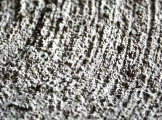
168 Figure A.1 Alpine Panel Figure A.2 Broom Drag PCC #1 Figure A.3 Broom Drag PCC #2 149

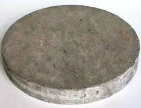
169 Figure A.4 Burlap Drag PCC #1 Figure A.5 Burlap Drag PCC #2 Figure A.6 Burlap Layover PCC #1 150

170 Figure A.7 Cheyenne Panel Figure A.8 Dense Grade Asphalt Concrete Figure A.9 Exposed Aggregate PCC #1 151

171 Figure A.10 Exposed Aggregate PCC #2 Figure A.11 Open (Coarse) Grade Asphalt Concrete #1 Figure A.12 Open (Coarse) Grade Asphalt Concrete #2 152

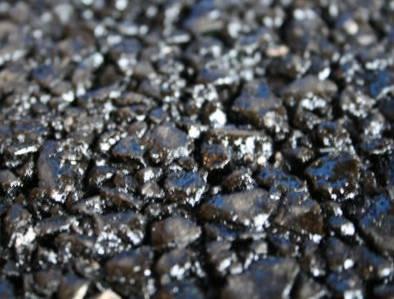
172 Figure A.13 Granite Stepping Stone Figure A.14 Rubber Stepping Stone Figure A.15 Stone Matrix Asphalt (SMA) Concrete #1 153

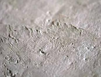
173 Figure A.16 Stone Matrix Asphalt (SMA) Concrete #2 Figure A.17 Smooth PCC #1 Figure A.18 Smooth PCC #2 154

174 Figure A Grit Sandpaper Figure A Grit Sandpaper Figure A Grit Sandpaper 155

175 Figure A.22 Radial Tine #1 Figure A.23 Radial Tine #2 Figure A.24 Tivoli Ceiling Tile 156

176 Figure A.25 Turf Drag PCC #1 Figure A.26 Turf Drag PCC #2 157

177 Appendix B CT Scan Supplemental Figures 158

178 B.1 Turf Drag PCC a.) b.) Figure B.1.1 Turf Drag PCC CT Scan Renderings a.) Top and b.) Side Views Figure B.1.2 Turf Drag PCC 2-D CT Scan Slice 159

179 Figure B.1.3 Turf Drag PCC 2-D CT Scan Slice Enhanced a.) b.) Figure B.1.4 Turf Drag PCC CT Scan Rendering a.) Top and b.) Side Views of 100 mm Square Sections 160

180 B.2 Dense Grade Asphalt Concrete a.) b.) Figure B.2.1 Dense Grade Asphalt Concrete CT Scan Renderings a.) Top and b.) Side Views Figure B.2.2 Dense Grade Asphalt Concrete 2-D CT Scan Slice 161

181 Figure B.2.3 Dense Grade Asphalt Concrete 2-D CT Scan Slice Enhanced a.) b.) Figure B.2.4 Dense Grade Asphalt Concrete CT Scan Rendering a.) Top and b.) Side Views of 100 mm Square Sections 162

182 B.3 Open Grade Asphalt Concrete a.) b.) Figure B.3.1 Open Grade Asphalt Concrete CT Scan Renderings a.) Top and b.) Side Views Figure B.3.2 Open Grade Asphalt Concrete 2-D CT Scan Slice 163

183 Figure B.3.3 Open Grade Asphalt Concrete 2-D CT Scan Slice Enhanced a.) b.) Figure B.3.4 Open Grade Asphalt Concrete CT Scan Rendering a.) Top and b.) Side Views of 100 mm Square Sections 164

184 Appendix C Sand Patch Data Sheets 165

185 Sample Test Volume Wt. D1 D2 D3 D4 Ave. Overall Ave. Overall Ave. MTD Ave. Number ml g in. in. in. in. in. in. mm mm Exposed Aggregate Broom Turf Drag Burlap Drag Alpine Tile Alpine Tile Open Grade Asphalt SMA Smooth

186 Sample Test Volume Wt. D1 D2 D3 D4 Ave. Overall Ave. Ave. MTD Overall Ave. Number ml g in. in. in. in. in. in. mm mm Exposed Agg Broom Turf Drag Burlap Drag Grit Sand paper Tivoli Panel (12") Grit Sand paper Grit Sand paper Burlap Layover

187 Sample Test Volume Wt. D1 D2 D3 D4 Ave. Overall Ave. Overall Ave. MTD Ave. Number ml g in. in. in. in. in. in. mm mm Smooth Turf Drag Smooth Granite Burlap Drag Radial Tine Radial Tine Cheyenne Tile Alpine Tile Exposed Aggregate

188 Sample Test Volume Wt. D1 D2 D3 D4 Ave. Overall Ave. Ave. Overall MTD Ave. Number ml g in. in. in. in. in. in. mm mm Exposed Aggregate Broom SMA Dense Grade Asphalt Open Grade Asphalt Rough Granite Grit Sandpaper Grit Sandpaper

189 Sample Test Volume Wt. D1 D2 D3 D4 Ave. Overall Ave. Ave. MTD Overall Ave. Number ml g in. in. in. in. in. in. mm mm Luna Panel Rubber Stepping Stone Burlap Drag Turf Drag Turf Drag Broom

190 Appendix D Ames Scanner Renderings vs. CT Scan Images 171

191 Figure D.1 Three-Dimensional Surface Rendering From Ames Scanner Dense Grade Asphalt Top and Side Views Figure D.2 Three-Dimensional Surface Rendering From CT Scan Dense Grade Asphalt Top and Side Views 172

192 Figure D.3 Three-Dimensional Surface Rendering From Ames Scanner Turf Drag PCC Top and Side Views Figure D.4 Three-Dimensional Surface Rendering From CT Scan Turf Drag PCC Top and Side Views 173

193 Figure D.5 Three-Dimensional Surface Rendering From Ames Scanner Open Grade Asphalt Top and Side Views Figure D.6 Three-Dimensional Surface Rendering From CT Scan Open Grade Asphalt Top and Side Views 174

194 Appendix E CT Meter Profiles 175

195 Figure E.1 50 Grit Sandpaper Profile Figure E.2 60 Grit Sandpaper Profile Figure E.3 80 Grit Sandpaper Profile Figure E.4 Alpine Panel Profile 176

196 Figure E.5 Broom 1 PCC Profile Figure E.6 Broom 2 PCC Profile Figure E.7 Burlap Drag 1 PCC Profile Figure E.8 Burlap Drag 2 PCC Profile 177

197 Figure E.9 Burlap Layover PCC Profile Figure E.10 Dense Grade Asphalt Profile Figure E.11 Exposed Aggregate 1 PCC Profile 178

198 Figure E.12 Exposed Aggregate 2 PCC Profile Figure E.13 Open Grade Asphalt 1 Profile 179

199 Figure E.14 Open Grade Asphalt 2 Profile Figure E.15 Radial Tine 1 Profile Figure E.16 Radial Tine 2 Profile 180

200 Figure E.17 Rough Granite Profile Figure E.18 Rubber Stepping Stone Profile Figure E.19 SMA 1 Profile 181

201 Figure E.20 SMA 2 Profile Figure E.21 Smooth 1 PCC Profile Figure E.22 Smooth 2 PCC Profile Figure E.23 Smooth Granite Profile 182

202 Figure E.24 Tivoli Tile Profile Figure E.25 Turf Drag 1 PCC Profile Figure E.26 Turf Drag 2 PCC Profile 183

203 Appendix F DFT Friction Coefficient Graphs 184

204 Figure F.1 Broom 1 PCC Graph Figure F.2 Broom 2 PCC Graph Figure F.3 Burlap Drag 1 PCC Graph 185

205 Figure F.4 Burlap Drag 2 PCC Graph Figure F.5 Burlap Layover PCC Graph Figure F.6 Dense Grade Asphalt Graph 186

206 Figure F.7 Exposed Aggregate 1 PCC Graph Figure F.8 Exposed Aggregate 2 PCC Graph Figure F.9 Open Grade Asphalt 1 Graph 187

207 Figure F.10 Open Grade Asphalt 2 Graph Figure F.11 Rubber Stepping Stone Graph Figure F.12 SMA 1 Graph 188

208 Figure F.13 SMA 2 Graph Figure F.14 Smooth 1 PCC Graph Figure F.15 Smooth 2 PCC Graph 189

209 Figure F.16 Radial Tine 1 PCC Graph Figure F.17 Radial Tine 2 PCC Graph Figure F.18 Turf Drag 1 PCC Graph 190

210 Figure F.19 Turf Drag 2 PCC Graph 191

211 Appendix G Supplemental Graphs, Tables, and Metric Equivalents 192

212 Certification Course Goodyear Test Track Sites Transportation Research Center Average MTD (in.) Standard Deviation (in.) COV Average ETD (in.) Standard Deviation (in.) COV Percent Diff. Smooth AC % % 40.9 Ground Asphalt Ground concrete Tined Concrete % % % % % % Chip Seal % % -301 Faulted Broken Concrete % % 10.6 Smooth AC % % 4.1 Tether Pad Genite Like 1984 AC Surface % % % % -1.3 Genite % % 24.4 Nova Chip % % Old Surface % % -0.3 Table G.1 (3.5M) Comparison of Average MTD and ETD Values for Each Pavement Type 193

213 50 Grit Sandpaper 60 Grit Sandpaper 1 80 Grit Sandpaper 1 Alpine Tile Sand Patch Ames Dynatest CT Meter Overall Average Average Average Average Average Average Average ETD ETD ETD ETD ETD ETD MTD 40 km/h 56 km/h 72 km/h 89 km/h mm mm (%) mm (%) mm (%) mm (%) mm (%) mm (%) (24.2) (49.3) (51.2) (57.7) (71.6) (30.7) (2.3) 0.43 (24.3) 0.41 (22.3) (17.9) (45.7) (51.8) (37.1) (68.6) (75.9) (76.7) (93.3) (41.5) (4.5) (0.0) (1.9) (12.5) (17.2) (19.3) Broom (21.7) (55.5) (54.3) (63.0) (55.6) (66.8) Broom (23.7) 0.81 (48.2) (52.4) (58.9) (51.4) (67.4) Burlap Drag 1 Burlap Drag 2 Burlap Layover Cheyenne Tile (2.6) (15.9) (22.2) (26.7) (12.5) (2.6) (13.5) (7.1) (11.4) (18.5) (6.0) (7.4) (27.1) (17.5) (28.3) (6.8) (15.1) (22.4) (32.2) - - Dense Grade Asphalt (10.0) (113.1) (65.1) Continued Table G.2 (11.1 M) MTD vs. Average ETD Percent Difference for Ames Laser Texture Scanner, Dynatest Laser Profiler at 40, 56, 72 and 89 km/h, and CT Meter [Values of Percent Difference in ( ) ] 194

214 Table G.2 Continued Sand Patch Ames Dynatest CT Meter Overall Average Average Average Average Average Average Average ETD ETD ETD ETD ETD ETD MTD 40 km/h 56 km/h 72 km/h 89 km/h mm mm (%) mm (%) mm (%) mm (%) mm (%) mm (%) Exposed Aggregate (28.6) (25.2) (29.2) (34.5) 1.67 (42.9) (23.6) 1 Exposed Aggregate (30.1) (23.9) (29.5) (31.4) (40.4) (36.8) 2 Open Grade (98.5) (83.8) Asphalt 1 Open Grade (135.5) (73.1) Asphalt 2 Radial Tine (20.8) (12.4) (20.0) (33.4) (40.7) (66.8) Radial Tine (21.6) (4.4) 2.13 (2.4) (12.3) (22.1) (91.5) Rough Granite (50.2) (50.0) (50.5) (44.5) (60.1) (27.3) Rubber Stepping Stone (102.6) (10.4) (32.5) (23.9) (109.0) SMA (57.7) (11.8) (53.6) SMA (35.5) (18.0) (19.2) Continued 195

215 Table G.2 Continued Smooth 1 Smooth 2 Smooth Granite Tivoli Panel (12") Turf Drag 1 Turf Drag 2 Sand Patch Ames Dynatest CT Meter Overall Average Average Average Average Average Average Average ETD ETD ETD ETD ETD ETD MTD 40 km/h 56 km/h 72 km/h 89 km/h mm mm (%) mm (%) mm (%) mm (%) mm (%) mm (%) (64.5) (65.8) (54.7) (58.0) (85.7) (63.7) (37.8) (44.1) (38.8) (36.3) (67.4) (5.7) (68.4) (102.5) (103.5) 0.39 (99.9) (120.9) (22.6) (37.2) (56.2) (54.4) (46.6) (75.2) (6.2) (11.5) (43.3) (43.9) (49.7) (41.8) (71.3) (13.7) (28.2) (31.7) (39.7) (34.2) (22.4) 196

216 Sample Type Concrete Non- Pavement Rough Samples Test Method Average Percent Difference Ames 24.40% Dynatest % Dynatest % Ames 31.50% Dynatest % Dynatest % Ames 25.90% Dynatest % Dynatest % Ames 49.00% Smooth Dynatest % Samples Dynatest % Table G.3 Percent Difference Comparison for Concrete Samples y = x R 2 = y = x R 2 = Coefficient of Friction y = x R 2 = y = x R 2 = ETD [mm] 20 km/h 40 km/h 60 km/h 80 km/h Linear (20 km/h) Linear (40 km/h) Linear (60 km/h) Linear (80 km/h) Figure G.1 (10.8M) CT Meter ETD versus Friction Coefficients at Varying Speeds 197

217 Open Grade Asphalt MTD [mm] Rubber Stepping Stone SMA MPD [mm] Figure G.2 Sand Patch MTD Versus Ames MPD with Outliers y = x R 2 = MTD [mm] MPD [mm] Figure G.3 Linear Relations and Coefficients of Correlation for Ames with No Outliers 198

218 y = x R 2 = ETD [mm] MPD [mm] Figure G.4 Linear Relations and Coefficients of Correlation for Dynatest Profiler at 40 km/h y = x R 2 = MTD [mm] MPD [mm] Figure G.5 Linear Relations and Coefficients of Correlation for Dynatest Profiler at 56 km/h 199

219 y = x R 2 = MTD [mm] MPD [mm] Figure G.6 Linear Relations and Coefficients of Correlation for Dynatest Profiler at 72 km/h y = x R 2 = MTD [mm] MPD [mm] Figure G.7 Linear Relations and Coefficients of Correlation for Dynatest Profiler at 89 km/h 200

220 MTD [mm] y = x R 2 = ETD = *MPD MPD [mm] Figure G.8 Overall Linear Relation and Coefficient of Correlation for Dynatest Profiler 201

221 202 MTD/ETD Values ASTM Sand Patch - MPD (mm) Standards Ames CT Meter Dynatest 25 Dynatest 35 Dynatest 45 Dynatest MPD Ames 0.8 MPD CT Meter Dynatest 40 km/h Dynatest 56 km/h MPD MPD MPD MPD MPD MPD MPD MPD R 2 = R 2 = R 2 = R 2 = R 2 = R 2 = MPD MPD MPD MPD MPD MPD R 2 = R 2 = R 2 = R 2 = R 2 = MPD MPD MPD MPD R 2 = R 2 = R 2 = R 2 = R 2 = MPD MPD MPD MPD MPD R 2 = R 2 = R 2 = R 2 = R 2 = MPD MPD MPD MPD MPD R 2 = R 2 = R 2 = R 2 = R 2 = Continued Table G.4 (11.4M) Comparison of Linear Relations and R 2 Values for MPD Measurements and ETD / MTD Values for All Methods 202

222 Table G.4 Continued 203 MTD/ETD Values Dynatest 72 km/h Dynatest 89 ASTM MPD (mm) Standards Ames CT Meter Dynatest 25 Dynatest 35 Dynatest 45 Dynatest MPD MPD MPD MPD MPD MPD R 2 = R 2 = R 2 = R 2 = R 2 = MPD MPD MPD MPD MPD km/h 0.8 MPD R 2 = R 2 = R 2 = R 2 = R 2 =

223 Ames ETD [in.] Radially Tined y = x R 2 = CT Meter MPD [in.] Figure G.9 Ames ETD versus CT Meter MPD Correlation with Outliers Radially Tined y = x R 2 = Ames ETD [mm] CT MPD [mm] Figure G.9M Ames ETD versus CT Meter MPD Correlation with Outliers 204

224 y = 0.826x R 2 = Ames ETD [in.] CT Meter MPD [in.] Figure G.10 Ames ETD versus CT Meter MPD Correlation without Outliers 2.50 Ames ETD [mm] y = 0.826x R 2 = CT MPD [mm] Figure G.10M Ames ETD versus CT Meter MPD Correlation without Outliers 205

225 y = x R 2 = Ames ETD [in.] Dynatest MPD [in.] Figure G.11 Ames ETD versus Dynatest MPD at 25 mph Correlation y = x R 2 = Ames ETD [mm] Dynatest MPD [mm] Figure G.11M Ames ETD versus Dynatest MPD at 40 km/h Correlation 206

226 y = x R 2 = Ames ETD [in.] Dynatest MPD [in.] Figure G.12 Ames ETD versus Dynatest MPD at 35 mph Correlation y = x R 2 = Ames ETD [mm] Dynatest MPD [mm] Figure G.12M Ames ETD versus Dynatest MPD at 56 km/h Correlation 207

227 y = x R 2 = Ames ETD [in.] Dynatest MPD [in.] Figure G.13 Ames ETD versus Dynatest MPD at 45 mph Correlation y = x R 2 = Ames ETD [mm] Dynatest MPD [mm] Figure G.13M Ames ETD versus Dynatest MPD at 72 km/h Correlation 208

228 y = x R 2 = Ames ETD [in.] Dynatest MPD [in.] Figure G.14 Ames ETD versus Dynatest MPD at 55 mph Correlation y = x R 2 = Ames ETD [mm] Dynatest MPD [mm] Figure G.14M Ames ETD versus Dynatest MPD at 89 km/h Correlation 209

229 CT Meter ETD [in.] y = x R 2 = Radially Tined Ames MPD [in.] Figure G.15 CT Meter ETD versus Ames MPD Correlation with Outliers CT Meter ETD [mm] y = x R 2 = Radially Tined Ames MPD [mm] Figure G.15M CT Meter ETD versus Ames MPD Correlation with Outliers 210

230 y = 0.833x R 2 = CT Meter ETD [in.] Ames MPD [in.] Figure G.16 CT Meter ETD versus Ames MPD Correlation without Outliers y = x R 2 = CT Meter ETD [mm] Ames MPD [mm] Figure G.16M CT Meter ETD versus Ames MPD Correlation without Outliers 211

231 CT Meter ETD [in.] y = x R 2 = Radially Tined Dynatest MPD [in.] Figure G.17 CT Meter ETD versus Dynatest MPD at 25 mph Correlation with Outliers CT Meter ETD [mm] y = x R 2 = Radially Tined Dynatest MPD [mm] Figure G.17M CT Meter ETD versus Dynatest MPD at 40 km/h Correlation With Outliers 212

232 0.10 CT Meter ETD [in.] y = x R 2 = Dynatest MPD [in.] Figure G.18 CT Meter ETD versus Dynatest MPD at 25 mph Correlation Without Outliers y = x R 2 = CT Meter ETD [mm] Dynatest MPD [mm] Figure G.18M CT Meter ETD versus Dynatest MPD at 40 km/h Correlation Without Outliers 213

233 CT Meter ETD [in.] y = x R 2 = Radially Tined Dynatest MPD [in.] Figure G.19 CT Meter ETD versus Dynatest MPD at 35 mph Correlation with Outliers 2.50 CT Meter ETD [mm] y = x R 2 = Radially Tined Dynatest MPD [mm] Figure G.19M CT Meter ETD versus Dynatest MPD at 56 km/h Correlation With Outliers 214

234 y = 0.884x R 2 = CT Meter ETD [in.] Dynatest MPD [in.] Figure G.20 CT Meter ETD versus Dynatest MPD at 35 mph Correlation Without Outliers 2.50 CT Meter ETD [mm] y = 0.884x R 2 = Dynatest MPD [mm] Figure G.20M CT Meter ETD versus Dynatest MPD at 56 km/h Correlation Without Outliers 215

235 CT Meter ETD [in.] y = x R 2 = Radially Tined Dynatest MPD [in.] Figure G.21 CT Meter ETD versus Dynatest MPD at 45 mph Correlation with Outliers 2.50 CT Meter ETD [mm] y = x R 2 = Radially Tined Dynatest MPD [mm] Figure G.21M CT Meter ETD versus Dynatest MPD at 72 km/h Correlation With Outliers 216

236 0.09 CT Meter ETD [in.] y = x R 2 = Dynatest MPD [in.] Figure G.22 CT Meter ETD versus Dynatest MPD at 45 mph Correlation Without Outliers 2.50 CT Meter ETD [mm] y = x R 2 = Dynatest MPD [mm] Figure G.22M CT Meter ETD versus Dynatest MPD at 72 km/h Correlation Without Outliers 217

237 CT Meter ETD [in.] y = x R 2 = Radially Tined Dynatest MPD [in.] Figure G.23 CT Meter ETD versus Dynatest MPD at 55 mph Correlation with Outliers CT Meter ETD [mm] y = x R 2 = Radially Tined Dynatest MPD [mm] Figure G.23M CT Meter ETD versus Dynatest MPD at 89 km/h Correlation With Outliers 218

238 CT Meter ETD [in.] y = x R 2 = Dynatest MPD [in.] Figure G.24 CT Meter ETD versus Dynatest MPD at 55 mph Correlation Without Outliers 2.50 CT Meter ETD [mm] y = x R 2 = Dynatest MPD [mm] Figure G.24M CT Meter ETD versus Dynatest MPD at 89 km/h Correlation without Outliers 219

239 Dynatest ETD [in.] y = x R 2 = y = x R 2 = y = x R 2 = y = x R 2 = Ames MPD [in.] 25 mph 35 mph 45 mph 55 mph Linear (25 mph) Linear (35 mph) Linear (45 mph) Linear (55 mph) Figure G.25 Dynatest ETD versus Ames MPD Correlations 2.50 Dynatest ETD [mm] y = x R 2 = y = x R 2 = y = x R 2 = y = x R 2 = Ames MPD [mm] 40 km/h 56 km/h 72 km/h 89 km/h Linear (40 km/h) Linear (56 km/h) Linear (72 km/h) Linear (89 km/h) Figure G.25M Dynatest ETD versus Ames MPD Correlations 220

240 y = 0.955x R 2 = Dynatest ETD [in.] y = x R 2 = y = x R 2 = y = x R 2 = CT Meter MPD [in.] 25 mph 35 mph 45 mph 55 mph Linear (25 mph) Linear (35 mph) Linear (45 mph) Linear (55 mph) Figure G.26 Dynatest ETD versus CT Meter MPD Correlations with Outliers 2.50 y = 0.955x R 2 = Dynatest ETD [mm] y = x R 2 = y = x R 2 = y = x R 2 = Ames MPD [mm] 40 km/h 56 km/h 72 km/h 89km/h Linear (40 km/h) Linear (56 km/h) Linear (72 km/h) Linear (89km/h) Figure G.26M Dynatest ETD versus CT Meter MPD Correlations with Outliers 221

241 y = x R 2 = Dynatest ETD [in.] y = x R 2 = y = x R 2 = y = x R 2 = CT Meter MPD [in.] 25 mph 35 mph 45 mph 55 mph Linear (25 mph) Linear (35 mph) Linear (45 mph) Linear (55 mph) Figure G.27 Dynatest ETD versus CT Meter MPD Correlations without Outliers 2.50 Dynatest ETD [mm] y = x R 2 = y = x y = x R 2 = R 2 = y = x R 2 = CT Meter MPD [mm] 40 km/h 56 km/h 72 km/h 89 km/h Linear (40 km/h) Linear (56 km/h) Linear (72 km/h) Linear (89 km/h) Figure G.27M Dynatest ETD versus CT Meter MPD Correlations without Outliers 222

242 y = x R 2 = ETD [in.] MPD [in.] Figure G.28 Dynatest ETD at 25 mph versus Dynatest MPD at 35 mph Correlation 2.50 ETD [mm] y = x R 2 = MPD [mm] Figure G.28M Dynatest ETD at 40 km/h versus Dynatest MPD at 56 km/h Correlation 223

243 y = x R 2 = ETD [in.] MPD [in.] Figure G.29 Dynatest ETD at 25 mph versus Dynatest MPD at 45 mph Correlation y = x R 2 = ETD [mm] MPD [mm] Figure G.29M Dynatest ETD at 40 km/h versus Dynatest MPD at 72 km/h Correlation 224

244 y = x R 2 = ETD [in.] MPD [in.] Figure G.30 Dynatest ETD at 25 mph versus Dynatest MPD at 55 mph Correlation y = x R 2 = ETD [mm] MPD [mm] Figure G.30M Dynatest ETD at 40 km/h versus Dynatest MPD at 89 km/h Correlation 225

245 y = x R 2 = ETD [in.] MPD [in.] Figure G.31 Dynatest ETD at 35 mph versus Dynatest MPD at 25 mph Correlation 2.50 ETD [mm] y = x R 2 = MPD [mm] Figure G.31M Dynatest ETD at 56 km/h versus Dynatest MPD at 40 km/h Correlation 226

246 y = 0.875x R 2 = ETD [in.] MPD [in.] Figure G.32 Dynatest ETD at 35 mph versus Dynatest MPD at 45 mph Correlation 2.50 ETD [mm] y = 0.875x R 2 = MPD [mm] Figure G.32M Dynatest ETD at 56 km/h versus Dynatest MPD at 72 km/h Correlation 227

247 y = x R 2 = ETD [in.] MPD [in.] Figure G.33 Dynatest ETD at 35 mph versus Dynatest MPD at 55 mph Correlation 2.50 ETD [mm] y = x R 2 = MPD [mm] Figure G.33M Dynatest ETD at 56 km/h versus Dynatest MPD at 89 km/h Correlation 228

248 y = x R 2 = ETD [in.] MPD [in.] Figure G.34 Dynatest ETD at 45 mph versus Dynatest MPD at 25 mph Correlation ETD [mm] y = x R 2 = MPD [mm] Figure G.34M Dynatest ETD at 72 km/h versus Dynatest MPD at 40 km/h Correlation 229

249 y = x R 2 = ETD [in.] MPD [in.] Figure G.35 Dynatest ETD at 45 mph versus Dynatest MPD at 35 mph Correlation ETD [mm] y = x R 2 = MPD [mm] Figure G.35M Dynatest ETD at 72 km/h versus Dynatest MPD at 56 km/h Correlation 230

250 y = x R 2 = ETD [in.] MPD [in.] Figure G.36 Dynatest ETD at 45 mph versus Dynatest MPD at 55 mph Correlation 2.50 ETD [mm] y = x R 2 = MPD [mm] Figure G.36M Dynatest ETD at 72 km/h versus Dynatest MPD at 89 km/h Correlation 231

251 y = x R 2 = ETD [in.] MPD [in.] Figure G.37 Dynatest ETD at 55 mph versus Dynatest MPD at 25 mph Correlation ETD [mm] y = x R 2 = MPD [mm] Figure G.37M Dynatest ETD at 89 km/h versus Dynatest MPD at 40 km/h Correlation 232

252 y = x R 2 = ETD [in.] MPD [in.] Figure G.38 Dynatest ETD at 55 mph versus Dynatest MPD at 35 mph Correlation ETD [mm] y = x R 2 = MPD [mm] Figure G.38M Dynatest ETD at 89 km/h versus Dynatest MPD at 56 km/h Correlation 233

253 y = x R 2 = ETD [in.] MPD [in.] Figure G.39 Dynatest ETD at 55 mph versus Dynatest MPD at 45 mph Correlation ETD [mm] y = x R 2 = MPD [mm] Figure G.39M Dynatest ETD at 89 km/h versus Dynatest MPD at 72 km/h Correlation 234

254 Sand Patch MTD [in.] CT Meter y = x R 2 = mph y = x R 2 = mph y = x R 2 = mph y = x R 2 = mph y = x R 2 = ETD [in.] CT M eter Dynatest 25 Dynatest 35 Dynatest 45 Dynatest 55 Linear (CT M eter) Linear (Dynatest 25) Linear (Dynatest 35) Linear (Dynatest 45) Linear (Dynatest 55) Linear (45 Degree) Figure G.40 Sand Patch MTD versus ETD from Ames Relations 3.00 Sand Patch MTD [mm] CT Meter y = x R 2 = Dyna 40 km/h y = x R 2 = Dyna 56 km/h y = x R 2 = Dyna 72 km/h y = x R 2 = Dyna 89 km/h y = x R 2 = ETD [mm] CT Meter Dynatest 40 Dynatest 56 Dynatest 72 Dynatest 89 Linear (CT Meter) Linear (Dynatest 40) Linear (Dynatest 56) Linear (Dynatest 72) Linear (Dynatest 89) Linear (45 Degree) Figure G.40M Sand Patch MTD versus ETD from Ames Relations 235

255 Sand Patch MTD [in.] Ames y = x R 2 = mph y = x R 2 = mph y = x R 2 = mph y = x R 2 = mph y = x R 2 = ETD [in.] Ames Dynatest 25 Dynatest 35 Dynatest 45 Dynatest 55 Linear (Ames) Linear (Dynatest 25) Linear (Dynatest 35) Linear (Dynatest 45) Linear (Dynatest 55) Linear (45 Degree) Figure G.41 Sand Patch MTD versus ETD from CT Meter Relations 3.00 Sand Patch MTD [mm] Ames y = x R 2 = Dyna 40 km/h y = x R 2 = Dyna 56 km/h y = x R 2 = Dyna 72 km/h y = x R 2 = Dyna 89 km/h y = x R 2 = ETD [mm] Ames Dynatest 40 Dynatest 56 Dynatest 72 Dynatest 89 Linear (Ames) Linear (Dynatest 40) Linear (Dynatest 56) Linear (Dynatest 72) Linear (Dynatest 89) Linear (45 Degree) Figure G.41M Sand Patch MTD versus ETD from CT Meter Relations 236

256 Sand Patch ETD [in.] Ames y = x R 2 = CT Meter y = x R 2 = mph y = x R 2 = mph y = x R 2 = mph y = 1.146x R 2 = ETD [in.] Ames CT M eter Dynatest 35 mph Dynatest 45 mph Dynatest 55 Linear (Ames) Linear (CT Meter) Linear (Dynatest 35 mph) Linear (Dynatest 45 mph) Linear (Dynatest 55) Linear (45 Degree) Figure G.42 Sand Patch MTD versus ETD from Dynatest at 25 mph Relations 3.00 Sand Patch ETD [mm] CT Meter y = x R 2 = Ames y = x R 2 = Dyna 56 km/h y = x R 2 = Dyna 72 km/h y = x R 2 = Dyna 89 km/h y = 1.146x R 2 = ETD [mm] Ames CT Meter Dynatest 56 Dynatest 72 Dynatest 89 Linear (Ames) Linear (CT Meter) Linear (Dynatest 56) Linear (Dynatest 72) Linear (Dynatest 89) Linear (45 Degree) Figure G.42M Sand Patch MTD versus ETD from Dynatest at 40 km/h Relations 237

257 0.12 Sand Patch MTD [in.] Ames y = x R 2 = CT Meter y = x R 2 = mph y = x R 2 = mph y = x R 2 = mph y = 1.205x R 2 = ETD [in.] Ames CT Meter Dynatest 25 mph Dynatest 45 mph Dynatest 55 Linear (Ames) Linear (CT Meter) Linear (Dynatest 25 mph) Linear (Dynatest 45 mph) Linear (Dynatest 55) Linear (45 Degree) Figure G.43 Sand Patch MTD versus ETD from Dynatest at 35 mph Relations 238

258 3.00 Sand Patch MTD [mm] Ames y = x R 2 = CT Meter y = x R 2 = Dyna 40 km/h y = x R 2 = Dyna 72 km/h y = x R 2 = Dyna 89 km/h y = 1.205x R 2 = ETD [mm] Ames CT Meter Dynatest 56 Dynatest 72 Dynatest 89 Linear (Ames) Linear (CT Meter) Linear (Dynatest 56) Linear (Dynatest 72) Linear (Dynatest 89) Linear (45 Degree) Figure G.43M Sand Patch MTD versus ETD from Dynatest at 56 km/h Relations Sand Patch MTD [in.] Ames y = x R 2 = CT Meter y = x R 2 = mph y = 1.281x R 2 = mph y = x R 2 = mph y = x R 2 = ETD [in.] Ames CT M eter Dynatest 25 Dynatest 35 Dynatest 55 Linear (Ames) Linear (CT M eter) Linear (Dynatest 25) Linear (Dynatest 35) Linear (Dynatest 55) Linear (45 Degree) Figure G.44 Sand Patch MTD versus ETD from Dynatest at 45 mph Relations 239

259 3.00 Sand Patch MTD [mm] Ames y = x R 2 = CT Meter y = x R 2 = Dyna 40 km/h y = 1.281x R 2 = Dyna 56 km/h y = x R 2 = Dyna 89 km/h y = x R 2 = ETD [mm] Ames CT Meter Dynatest 40 Dynatest 56 Dynatest 89 Linear (Ames) Linear (CT Meter) Linear (Dynatest 40) Linear (Dynatest 56) Linear (Dynatest 89) Linear (45 Degree) Figure G.44M Sand Patch MTD versus ETD from Dynatest at 72 km/h Relations Sand Patch MTD [in.] Ames y = 1.395x R 2 = CT Meter y = x R 2 = mph y = x R 2 = mph y = x R 2 = mph y = x R 2 = ETD [in.] Ames Dynatest 25 mph Dynatest 45 mph Linear (CT Meter) Linear (Dynatest 35 mph) Linear (45 Degree) CT M eter Dynatest 35 mph Linear (Ames) Linear (Dynatest 25 mph) Linear (Dynatest 45 mph) Figure G.45 Sand Patch MTD versus ETD from Dynatest at 55 mph Relations 240

260 3.00 Sand Patch MTD [mm] Ames y = x R 2 = CT Meter y = x R 2 = Dyna 40 km/h y = x R 2 = Dyna 56 km/h y = x R 2 = Dyna 72 km/h y = x R 2 = ETD [mm] Ames CT Meter Dynatest 40 Dynatest 56 Dynatest 72 Linear (Ames) Linear (CT Meter) Linear (Dynatest 40) Linear (Dynatest 56) Linear (Dynatest 72) Linear (45 Degree) Figure G.45M Sand Patch MTD versus ETD from Dynatest at 89 km/h Relations Ames y = x R 2 = CT Meter y = x R 2 = Dyna 40 km/h y = x R 2 = MTD [mm] Dyna 72 km/h y = x R 2 = Dyna 56 km/h y = x R 2 = Dyna 89 km/h y = x R 2 = ETD [mm] Ames CT Meter Dynatest 40 Dynatest 56 Dynatest 72 Dynatest 89 Linear (Ames) Linear (CT Meter) Linear (Dynatest 40) Linear (Dynatest 56) Linear (Dynatest 72) Linear (Dynatest 89) Figure G.46 (11.10M) Sand Patch MTD versus ETD from Sand Patch Relations 241

261 Appendix H Supplemental Photos 242

262 Figure H.1 Concrete Molds Figure H.2 Mixing of Concrete Used for Samples Figure H.3 Broom Drag PCC Sample in Mold With Broom Used for Finishing 243

263 Figure H.4 Turf Drag PCC Sample in Mold With Turf Used for Finishing Figure H.5 Exposed Agg. PCC Sample in Mold After Top Mortar Removal With Water Figure H.6 Asphalt Samples After Fabrication at Kokosing Materials Laboratory in Mansfield, OH 244

264 Figure H.7 14-in. Metal Ring Used for Fabricating Asphalt Samples Metal Ring Cut From 14-in. Diameter Metal Drum Figure H.8 SMA Asphalt Sample With Restraining Collar Made From Hose Clamps Riveted to Sheet Metal 245

265 Figure H.9 Wheel Path View of Testing Apparatus Figure H.10 Top Down View of Test Apparatus Figure H.11 Ames Scanner Laser Dot on Samples 246