FINAL REPORT FHWA/IN/JTRP-2004/12. Quality Control Procedures for Weigh-in-Motion data. Andrew P. Nichols Graduate Research Assistant

Transcription

1 FINAL REPORT FHWA/IN/JTRP-2004/12 Quality Control Procedures for Weigh-in-Motion data By Andrew P. Nichols Graduate Research Assistant Darcy M. Bullock Professor School of Civil Engineering Purdue University Joint Transportation Research Program Project No: C-36-17MMM File No: SPR Conducted in Cooperation with the Indiana Department of Transportation and the U.S. Department of Transportation Federal Highway Administration The contents of this report reflect the views of the authors, who are responsible for the facts and the accuracy of the data presented herein. The contents do not necessarily reflect the official views or policies of the Indiana Department of Transportation or the Federal Highway Administration at the time of publication. The report does not constitute a standard, specification, or regulation. Purdue University West Lafayette, IN June 2004

2 INDOT Research TECHNICAL Summary Technology Transfer and Project Implementation Information TRB Subject Code: 53-9 Weigh-in-Motion June 2004 Publication No.: FHWA/IN/JTRP-2004/12, SPR-2795 Final Report Quality Control Procedures for Weigh-in-Motion Data Introduction For the past two decades, weigh-in-motion (WIM) sensors have been used in the United States to collect vehicle weight data for designing pavements and monitoring their performance. The use of these sensors is being expanded for enforcement purposes to screen vehicles in traffic streams for overweight violations. This screening procedure is broadly referred to as a virtual weigh station. WIM sensors are also used at static weigh stations for screening vehicles to be stopped and weighed statically, resulting in reduced driver delay and increased efficiency by only weighing trucks that are close to the legal weight limit. The effectiveness of static weigh stations in Indiana for identifying overweight trucks has not been previously documented. Therefore, it was not possible to determine if the virtual weigh stations were a more effective tool and warrant widespread deployment across the state. Findings This study found that static weigh stations in Indiana were effective for identifying safety violations, but ineffective for identifying overweight vehicles. It was also determined that the virtual weigh stations in Indiana were found to be approximately 55 times more effective than the static weigh stations for overweight truck identification. To achieve that level of effectiveness, the virtual weigh stations require a high level of WIM data accuracy and reliability that can only be attained with a rigorous quality control program. Accurate WIM data is also essential to the success of the Long-term Pavement Performance project and the development of new pavement design methods. Robust metrics were identified for the quality control program that can be continuously The WIM enforcement applications require a high level of data accuracy for optimal performance. This level of accuracy has been difficult to achieve with the traditional planning and design applications because the data is aggregated and not scrutinized for individual vehicles. If the WIM sensor is weighing too light, illegal trucks may not be identified reducing the enforcement effectiveness. If the WIM sensor is weighing too heavy, legal trucks may be identified as overweight reducing the enforcement efficiency. This project was initiated to develop a quality control program for the Indiana Department of Transportation (INDOT) to improve the accuracy of the data produced from the WIM system. The quality control program provides a mechanism for assessing the accuracy of vehicle classification, weight, speed, and axle spacing data and monitoring it over time. monitored using statistical process control procedures that differentiate between sensor noise and events that require intervention. The speed and axle spacing accuracy is assessed by examining the drive tandem axle spacing of the Class 9 vehicle. The population average of this metric should range between 4.30 and 4.36 feet. The weight accuracy is assessed by examining the total steer axle weight and left-right steer axle residual of the Class 9 vehicle population. The population average steer axle weight should range between 9,000 and 11,000 lbs depending on the percentage of loaded vehicles. The population average left-right residual should range between - 6% and +6% depending on the cross-slope of the roadway. The sensor error rates can be assessed and monitored by computing the proportion of errors relative to the number of vehicles /04 JTRP-2004/12 INDOT Division of Research West Lafayette, IN 47906

3 An example of the accuracy and monitoring reports developed in this project for the speed accuracy, weight accuracy, and error rates are depicted in Figure 1, Figure 2, and Figure 3, respectively. The system accuracy charts (Figure 1a, Figure 2a, Figure 3a) include the average values for each WIM lane in the entire system. If a lane s value is outside of the target range, a statistical process control chart (Figure 1b, Figure 2b, Figure 3b) for that lane is used to determine if the deviation is attributed to random variation or a sensor problem. Data mining of the accuracy metrics revealed variations in the data caused by sensor failure and sensor drift, sometimes attributed to temperature and precipitation, and incorrect calibration. The statistical process control charts revealed that the WIM sensor measurements are not in statistical control and frequently drift out of calibration. To establish and maintain accurate data, the WIM data should be continuously monitored for errors and drifts. It is also recommended that the system algorithms consider variations in the climate to account for temperature and precipitation or flag data that is collected during days of climatic anomalies when the accuracy is questionable. Implementation This report developed a set of tools that the Indiana Department of Transportation can use to assess WIM data accuracy and monitor that accuracy over time. Implementing the following items will establish and make use of these tools to improve the overall accuracy of the WIM systems in Indiana: Implement procedures for importing WIM data into a relational database. This will facilitate the creation of the analysis cube files that are essential for data manipulation and exploration. Apply the drive tandem axle spacing metric to all WIM systems to monitor the speed calibration and prioritize maintenance on a lane basis. For lanes with poor speed calibration, approximate the calibration using the average drive tandem axle spacing metric prior to field calibration using a laser gun. Apply the error proportion metric to all WIM systems to identify lanes that experience high error rates to prioritize maintenance on a lane basis. Configure bending plate and single load cell WIM systems to log the left and right wheel data to compute the left-right residual metric. Use the left-right residual for detecting weight calibration drift and to prioritize maintenance on a lane basis. Construct a test bed of various types of WIM sensors for a long-term evaluation of performance, accuracy, and maintenance costs for each type. Installation of necessary equipment to collect continuous climate data adjacent to the test bed would allow further exploration of the climatic impacts on the WIM sensors. Contacts For more information: Prof. Darcy Bullock Principal Investigator School of Civil Engineering Purdue University West Lafayette IN Phone: (765) Fax: (765) darcy@purdue.edu Indiana Department of Transportation Division of Research 1205 Montgomery Street P.O. Box 2279 West Lafayette, IN Phone: (765) Fax: (765) Purdue University Joint Transportation Research Program School of Civil Engineering West Lafayette, IN Phone: (765) Fax: (765) jtrp@ecn.purdue.edu /04 JTRP-2004/12 INDOT Division of Research West Lafayette, IN 47906

4 Average Drive Tandem Axle Spacing (feet) feet Average (feet) Average Standard Deviation Std Dev (feet) WIM Lane 10/01/ /08/ /15/ /22/ /29/ /05/ /12/ /19/ /26/ /03/ /10/ /17/ /24/ /31/2003 a) System Accuracy Chart b) Statistical Process Control Chart Figure 1. Speed Quality Control % Subgroup Average 27% Average Front Axle Weight (lbs) ,000 to 11,000 lbs Average 3% 0% -3% -6% -9% -12% Subgroup Standard Deviation 24% 21% 18% 15% 12% 9% 6% Std Dev -15% 3% 0 WIM Lane 08/01/ /08/ /15/ /22/ /29/ /05/ /12/ /19/ /26/ /03/ /10/ /17/ /24/ /31/ /07/ /14/ /21/ /28/ /05/2003 a) System Accuracy Chart b) Statistical Process Control Chart Figure 2. Weight Quality Control 100% 50% 90% 80% 40% Thanksgiving Christmas Memorial Day Thanksgiving Christmas Error Rate 70% 60% 50% 40% Error Proportion 30% 20% 30% 20% 10% 10% 0% 0% WIM Lane 09/01/ /01/ /01/ /01/ /01/ /01/ /01/ /01/ /01/ /01/ /01/ /01/ /01/ /01/ /01/ /01/2003 a) System Accuracy Chart b) Statistical Process Control Chart Figure 3. Error Rate Quality Control /04 JTRP-2004/12 INDOT Division of Research West Lafayette, IN 47906

5 1. Report No. 2. Government Accession No. 3. Recipient's Catalog No. FHWA/IN/JTRP-2004/12 TECHNICAL REPORT STANDARD TITLE PAGE 4. Title and Subtitle Quality Control Procedures for Weigh-in-Motion Data 5. Report Date June Performing Organization Code 7. Author(s) Andrew P. Nichols and Darcy M. Bullock 9. Performing Organization Name and Address Joint Transportation Research Program 550 Stadium Mall Drive Purdue University West Lafayette, IN Performing Organization Report No. FHWA/IN/JTRP-2004/ Work Unit No. 11. Contract or Grant No. SPR Sponsoring Agency Name and Address Indiana Department of Transportation State Office Building 100 North Senate Avenue Indianapolis, IN Type of Report and Period Covered Final Report 14. Sponsoring Agency Code 15. Supplementary Notes Prepared in cooperation with the Indiana Department of Transportation and Federal Highway Administration. 16. Abstract For the past two decades, weigh-in-motion (WIM) sensors have been used in the United States to collect vehicle weight data for designing pavements and monitoring their performance. The use of these sensors is now being expanded for enforcement purposes to provide virtual weigh stations for screening vehicles in traffic streams for overweight violations. A study found that static weigh stations in Indiana were effective for identifying safety violations, but ineffective for identifying overweight vehicles. It was also determined that the alternative approach to identifying overweight vehicles using virtual weigh stations requires a high level of WIM data accuracy and reliability that can only be attained with a rigorous quality control program. Accurate WIM data is also essential to the success of the Long-term Pavement Performance project and the development of new pavement design methods. This report proposes a quality control program that addresses vehicle classification, speed, axle spacing, and weight accuracy by identifying robust metrics that can be continuously monitored using statistical process control procedures that differentiate between sensor noise and events that require intervention. The speed and axle spacing accuracy is assessed by examining the drive tandem axle spacing of the population of Class 9 vehicles. The weight accuracy is assessed by examining the left-right steer axle residual weight of the population of Class 9 vehicles. Data mining of these metrics revealed variations in the data caused by incorrect calibration, sensor failure, temperature, and precipitation. The accuracy metrics could be implemented in a performance-based specification for WIM systems that is more feasible to enforce than the current specifications based on comparing static vehicle weights with dynamic vehicle weights measured by the WIM sensors. The quality control program can also be used by agencies to prioritize maintenance to more effectively allocate the limited funds available for sensor repair and calibration. This research provides a tool that agencies can use to obtain and sustain higher quality WIM data. 17. Key Words Weigh-in-motion, virtual weigh station, static weigh station, weight enforcement, quality control, statistical process control, data mining. 18. Distribution Statement No restrictions. This document is available to the public through the National Technical Information Service, Springfield, VA Security Classif. (of this report) 20. Security Classif. (of this page) 21. No. of Pages 22. Price Unclassified Unclassified 239 Form DOT F (8-69)

6 TABLE OF CONTENTS LIST OF TABLES...vi LIST OF FIGURES... viii IMPLEMENTATION REPORT...xii ACKNOWLEDGMENTS... xiii CHAPTER 1. INTRODUCTION Traditional WIM Applications Evolving WIM Applications Commercial Vehicle Enforcement Pavement Design Current WIM Data Accuracy Data Quality Control Program History Six Sigma Process Truck Characteristics Summary CHAPTER 2. PROBLEM STATEMENT DEFINITION Introduction I-80/94 WIM Data Summary Pavement Life Overweight Truck Distributions Static Weigh Station Study Data Collection Equipment and Driver Violations Weight Violations Temporal Distribution of Violations Weigh Station Open/Close Analysis Hazard-based Duration Models Trucks with Gross Vehicle Weight OEV Trucks with Gross Vehicle Weight < 85,000 lbs Virtual Weigh Station Comparison Summary CHAPTER 3. DEFINITION OF IMPROVEMENT GOALS Introduction WIM Accuracy Standard Improvement Goals CHAPTER 4. SPEED ACCURACY METRIC Introduction Truck Characteristics WIM Calculations WIM Speed WIM Axle Spacing Speed Calibration Calibration Errors WIM Error Relationships iii

7 4.4. Speed and Axle Spacing Relationship Site Selection Data Collection Regression Analysis Car and Truck Speed Comparison Data Analysis Case Study: Impact of Speed Error on Classification Accuracy Plots Summary CHAPTER 5. WEIGHT ACCURACY METRIC Introduction Truck Characteristics Weight Assessment Metric for Data Mining Weight Monitoring Metric for Accuracy Monitoring Derivation Cross-slope Correction Interpretation Data Analysis Piezoelectric Sensor Weight Accuracy Summary CHAPTER 6. DATA COLLECTION & PROCESSING Introduction Data Transformation Database Design Analysis Tools Summary CHAPTER 7. DATA MINING & ROOT CAUSE ANALYSIS Introduction WIM Errors and Warnings Case Study: Site Case Study: Site Case Study: Site Case Study: Site Summary CHAPTER 8. SOLUTIONS & IMPLEMENTATION Introduction Approximate Calibration Tuning Approximate Speed Calibration Approximate Weight Calibration Climate Solutions Implementation Summary CHAPTER 9. DOCUMENTATION, PROCESS MONITORING, & POLICY CHANGES Introduction Documentation Statistical Process Control Control Chart Basics Overview Subgroup Frequency Subgroup Sample Size Random Sampling Average and Standard Deviation Charts Moving Average and Moving Standard Deviation Charts Plots iv

8 Rules Class 9 Drive Tandem Axle Spacing Characteristics Sample Size Average and Standard Deviation Charts Moving Average and Moving Standard Deviation Assignable Causes Class 9 Steer Axle Left-Right Residual Characteristics Sample Size Average and Standard Deviation Charts Moving Average and Moving Standard Deviation Assignable Causes Error Counts P-Charts Assignable Causes Policy Changes Summary CHAPTER 10. CONCLUSIONS Summary Contributions Recommendations WIM System Modifications WIM Standard Modifications Future Research LIST OF REFERENCES Appendix A. Indiana WIM Sites Appendix B. FHWA Scheme F Vehicle Classification Scheme Appendix C. Static Weigh Station Study Results v

9 LIST OF TABLES Table 2.1 I-80/94 Class 9 ESAL Projections for Lane Table 2.2 I-80/94 Class 9 ESAL Projections for Lane Table 2.3 I-80/94 Class 9 Gross Vehicle Weight Statistics May 2002-April Table 2.4 I-80/94 Class 9 Tandem Weight Statistics May 2002-April Table 2.5 Indiana Static Weigh Stations Table 2.6 Violation Codes Table 2.7 Gross Vehicle Weight Violations 85,000 lbs at Indiana Static Weigh Stations August- September Table 2.8 Weigh Station Analysis Weeks Table 2.9 LIMDEP Output Week 1 Weibull Model Table 2.10 LIMDEP Log-likelihood at Convergence Values Table 2.11 Weibull P Parameter Significance Table 2.12 Weibull and Exponential Model Significance Test Table 2.13 Weibull and Log Logistic Model Significance Test Table 2.14 Weekly Chi-square Comparisons Table 2.15 Weekly Difference Significance Levels Table 2.16 LIMDEP Output Week 1 Weibull Model Table 2.17 LIMDEP Log-likelihood at Convergence Values Table 2.18 Weibull P Parameter Significance Table 2.19 Weibull and Log Logistic Model Significance Test Table 2.20 Weekly Chi-square Comparisons Table 2.21 Weekly Difference Significance Levels Table 2.22 Virtual Weigh Station Activity Table 3.1 ASTM E WIM Categories Table 3.2 Data Items Produced by WIM System Table 3.3 ASTM E WIM Accuracy Tolerances for 95% Probability of Conformity Table 3.4 ASTM E Static Weight Tolerances...66 Table Truck Manufacturer Sales by Drive Tandem Axle Spacing Table 4.2 Class 9 Drive Tandem Axle Spacing Target Values Table 4.3 Class 9 vs. Non-Class 9 Speed Analysis Table 4.4 WIM Vendor FHWA Classification File for Vehicles with 5 Axles Table 4.5 Class 9 Data from Raw Data File WIM Site Table 4.6 Average Drive Tandem Axle Spacing Comparison WIM Site Table 4.7 Class 9 Data from Raw Data File WIM Site Table 5.1 Class 9 Steer Axle Weight Target Values Table 5.2 Sample Data Illustrating Left-Right Residual Table 5.3 Left-Right Residual Caused by Roadway Cross-slope Table 5.4 Left-Right Residual Trends Table 6.1 Sample Indiana WIM Raw Record Files for a Class 9 Truck Table 6.2 WIM Database Size Table 6.3 Analysis Cube File Attributes and Size Table 7.1 Vendor WIM Error and Warning Description Table 9.1 Control Chart Coefficients Table 9.2 Probability of Rule Violations vi

10 Table 9.3 Site 4700 Lane 1 Drive Tandem Axle Spacing Data Table 9.4 Site 4700 Lane 3 Drive Tandem Axle Spacing Data Table 9.5 Drive Tandem Axle Spacing Control Limits Table 9.6 Sample Subgroup Left-Right Residual Average and Standard Deviation Table 9.7 Left-Right Residual Control Limits for Site 3520 Lane 2 and Lane Table 9.8 Error Proportion P-Chart Limits Table A.1 Indiana WIM Site Summary vii

11 LIST OF FIGURES Figure 1.1 Transponder Program Infrastructure... 2 Figure 1.2 Weigh Station Sorting Lane... 3 Figure 1.3 Virtual Weigh Station Photo Enforcement... 4 Figure 1.4 Mobile Enforcement Weight Measurement... 4 Figure 1.5 Virtual Weigh Station Software... 5 Figure 1.6 Virtual Weigh Station Enforcement Data... 7 Figure 1.7 DMAIC Performance Improvement Model Figure 2.1 WIM Sites 4000 and 4010 on I-80/94 at Milepost Figure 2.2 ESAL Calculation for Class 9 Trucks Figure 2.3 Total ESAL by Lane May 2002-April Figure 2.4 I-80/94 ESAL Projections Eastbound Lane Figure 2.5 I-80/94 ESAL Projections Westbound Lane Figure 2.6 I-80/94 ESAL Projections Eastbound Lane Figure 2.7 I-80/94 ESAL Projections Westbound Lane Figure 2.8 Indiana Static Weigh Stations Figure 2.9 Sample Violation Log Figure 2.10 Violations at All Indiana Static Weigh Stations August-September Figure 2.11 Weight Violation Count at Indiana Static Weigh Stations August-September Figure 2.12 Ticket Distributions at Indiana Static Weigh Stations August-September Figure 2.13 Warning Distributions at Indiana Static Weigh Stations August-September Figure 2.14 Tandem Weight Violations at Indiana Static Weigh Stations August-September Figure 2.15 Gross Vehicle Weight Violations at Indiana Static Weigh Stations August-September Figure 2.16 Hourly Weight Ticket Distribution by Elapsed Open Time Active Weigh Stations Figure 2.17 Hourly Weight Ticket Distribution by Time of Day Active Weigh Stations Figure 2.18 I-74 Weigh Station and WIM Figure 2.19 Veedersburg Weigh Station Open Hours...40 Figure 2.20 Truck Arrival Count Figure 2.21 Truck Arrival Cumulative Distribution Figure 2.22 Cumulative Distribution Functions for Week 1 Models Figure 2.23 Hazard Functions for Week 1 Models Figure 2.24 Weibull Cumulative Distribution Functions Figure 2.25 Weibull Hazard Functions for All Weeks Figure 2.26 Truck Arrival Count Figure 2.27 Truck Arrival Cumulative Distribution Figure 2.28 Cumulative Distribution Functions for Week 1 Models Figure 2.29 Hazard Functions for Week 1 Models Figure 2.30 Weibull Cumulative Distribution Functions Figure 2.31 Weibull Hazard Functions for All Weeks Figure 2.32 Weibull Cumulative Distribution Functions for All Trucks and All Weeks Figure 2.33 Weibull Hazard Functions for All Trucks and All Weeks Figure 2.34 Overweight Activity Chart Figure 3.1 ASTM Test Vehicle Types Figure 3.2 Site 2400 Lane 1 Pavement Profile Figure 4.1 Class 9, 10, 12, 13 Tractor viii

12 Figure 4.2 Speed Error Estimate Figure 4.3 Typical Indiana Weigh-in-Motion Site Layout Figure 4.4 Side View of Single Load Cell Sensor Figure 4.5 Piezoelectric Axle Sensor Replacement Figure 4.6 Speed Sensor Distance Measurement Tolerances for ASTM Compliance at 65 mph Figure 4.7 Laser Gun Speed Data Correction Figure 4.8 Class 9 vs. Non-Class 9 Speed Comparison Figure 4.9 WIM Site 1200 Speed Accuracy Figure 4.10 WIM Site 1200 Drive Tandem Axle Spacing Histogram Figure 4.11 WIM Site 4200 Speed Accuracy Figure 4.12 WIM Site 4200 Drive Tandem Axle Spacing Histogram Figure 4.13 WIM Site 4700 Speed Accuracy Figure 4.14 WIM Site 4700 Drive Tandem Axle Spacing Histogram Figure 4.15 Class 9 Drive Tandem Axle Spacing Distribution WIM Site Figure 4.16 WIM Site 4200 Lane 1 Unclassified Count and Drive Tandem Axle Spacing Figure 4.17 WIM Site 4200 Lane 1 Unclassified Vehicle Axle 3-4 Spacing Histogram Figure 4.18 Average Drive Tandem Axle Spacing for All Indiana WIM Lanes April Figure 5.1 Steer Axle and Gross Vehicle Weight Relationship at Florida Weigh Station Figure 5.2 Steer Axle and Axle 1-2 Spacing Relationship at Florida Weigh Station Figure 5.3 Roadway Cross-Slope Dynamics Figure 5.4 California Bending Plate Site Steer Axle Left-Right Residual Figure 5.5 California Bending Plate Lane 4 Steer Axle Left-Right Residual vs. Steer Axle Weight Figure 5.6 California Bending Plate Lane 4 All Axles Left-Right Residual Figure 5.7 Site 3520 Steer Axle Left-Right Residual Figure 5.8 Indiana Single Load Cell Site 3520 Lane 2 Steer Axle Left-Right Residual vs. Weight Figure 5.9 Indiana Single Load Cell Site 3520 Lane 3 Steer Axle Left-Right Residual vs. Weight Figure 5.10 Indiana Single Load Cell Site 3520 Lane 2 All Axles Left-Right Residual Figure 5.11 Indiana Single Load Cell Site 3520 Lane 3 All Axles Left-Right Residual Figure 6.1 Data Processing Diagram Figure 6.2 Database Schema Figure 6.3 Analysis Cube Concept Figure 7.1 Piezoelectric Sensor Axle Detection Figure 7.2 Monthly Average Drive Tandem Axle Spacing Site Figure 7.3 Daily Average Drive Tandem Axle Spacing Site Figure 7.4 Hourly Average Drive Tandem Axle Spacing Site Figure 7.5 Site 4200 Log File Excerpt Figure 7.6 Site 4200 Piezoelectric Sensor Installations Figure 7.7 Hourly Average Drive Tandem Axle Spacing Site Figure 7.8 Site 4200 Log File Excerpt Figure 7.9 Monthly Class 9 Count Site 4200 All Lanes Figure 7.10 Daily Average Class 9 Speed Site 4200 All Lanes Figure 7.11 Hourly Average Drive Tandem Axle Spacing Site Figure 7.12 Site 4200 Lane 1 Error and Warning Counts Figure 7.13 Site 4200 Lane 1 Tandem Axle Spacing and Steer Axle Weight Figure 7.14 Site 4200 Lane 1 Daily Average Steer Axle Weight and Minimum Temperature Figure 7.15 Site 4700 Monthly Average Drive Tandem Axle Spacing Figure 7.16 Site 4700 Daily Average Drive Tandem Axle Spacing Figure 7.17 Site 4700 Lane 1 Monthly Error Count Figure 7.18 Site 4700 Lane 3 Monthly Error Count Figure 7.19 Site 4700 Log File Excerpt Figure 7.20 Site 4700 Lane 1 Error Count and Minimum Temperature Figure 7.21 Site 4700 Lane 3 Error Count and Minimum Temperature Figure 7.22 Site 4700 Lane 3 Error Rate and Precipitation Figure 7.23 Site 4000 Monthly Average Steer Axle Weight ix

13 Figure 7.24 Site 4000 Lane 4 Error Type 19 Count Figure 7.25 Site 4000 Lane 4 Error Rate and Minimum Temperature Figure 7.26 Site 4000 Daily Average Steer Axle Weight Figure 7.27 Site 4000 Log File Excerpt Figure 7.28 Site 4000 Class 4-13 Volume and Error Rates Figure 7.29 Site 4000 Lane 2 Error Type 13 Count Figure 7.30 Site 4000 Daily Maximum Temperature and Precipitation Figure 7.31 Site 3520 Daily Average Left-Right Residual Figure 7.32 Site 3520 Class 9 Volumes Figure 7.33 Site 3520 Lane 3 Daily Average Left-Right Residual and Minimum Temperature Figure 7.34 Site 3520 Daily Average Drive Tandem Axle Spacing Figure 7.35 Site 3520 Log File Excerpt Figure 7.36 Site 3520 Monthly Error Type 13 Counts and Class 4-13 Volumes Figure 8.1 Average Drive Tandem Axle Spacing All Lanes May Figure 8.2 Average Steer Axle Weight All Lanes May Figure 8.3 Autocalibration Bins Figure 8.4 Site 4700 Daily Average Steer Axle Weight (Piezoelectric Sensor) Figure 8.5 Site 3520 Daily Average Steer Axle Weight by Lane (Load Cell Sensor) Figure 8.6 Site 4700 Lane 1 Daily Average Steer Axle Weight Autocalibration Comparison Figure 8.7 Indiana Average Drive Tandem Axle Spacing for Maintained Lanes in Figure 8.8 Indiana Average Steer Axle Weight for Maintained Lanes in Figure 9.1 Area Under Normal Distribution Curve Figure 9.2 Sample Average Control Chart Figure 9.3 Sample Average Control Chart with Zones Figure 9.4 Western Electric Rule Illustration Figure Sales Histogram Figure 9.6 Site 4700 Drive Tandem Axle Spacing Histogram 4/1/03-4/7/ Figure 9.7 Site 4700 Lane 1 Average and Standard Deviation Control Chart for Drive Tandem Spacing Figure 9.8 Site 4700 Lane 2 Average and Standard Deviation Control Chart for Drive Tandem Spacing Figure 9.9 Site 4700 Lane 3 Average and Standard Deviation Control Chart for Drive Tandem Spacing Figure 9.10 Site 4700 Lane 4 Average and Standard Deviation Control Chart for Drive Tandem Spacing Figure 9.11 Site 4700 Lane 1 Moving Average and Standard Deviation for Drive Tandem Spacing Figure 9.12 Site 4700 Lane 2 Moving Average and Standard Deviation for Drive Tandem Spacing Figure 9.13 Site 4700 Lane 3 Moving Average and Standard Deviation for Drive Tandem Spacing Figure 9.14 Site 4700 Lane 4 Moving Average and Standard Deviation for Drive Tandem Spacing Figure 9.15 Site 3520 Left-Right Residual Histogram Figure 9.16 Site 3520 Lane 2 Control Chart for Left-Right Residual Figure 9.17 Site 3520 Lane 3 Control Chart for Left-Right Residual Figure 9.18 Site 3520 Lane 2 Moving Average and Standard Deviation for Left-Right Residual Figure 9.19 Site 3520 Lane 3 Moving Average and Standard Deviation for Left-Right Residual Figure 9.20 Site 4700 Lane 1 P-Chart Figure 9.21 Site 4700 Lane 2 P-Chart Figure 9.22 Site 4700 Lane 3 P-Chart Figure 9.23 Site 4700 Lane 4 P-Chart Figure 9.24 Site 4700 Lane 2 P-Chart Including Weekends Figure 9.25 Speed Quality Control Figure 9.26 Weight Quality Control Figure 9.27 Error Rate Quality Control Figure 10.1 Redundant Sensor Testing Layout Figure B.1 FHWA Class 1: Motorcycles x

14 Figure B.2 FHWA Class 2: Passenger Cars (With 1- or 2-Axle Trailers) Figure B.3 FHWA Class 3: 2 Axles, 4-Tire Single Units, Pickup or Van (With 1- or 2-Axle Trailers) Figure B.4 FHWA Class 4: Buses Figure B.5 FHWA Class 5: 2D - 2 Axles, 6-Tire Single Units (Includes Handicap-Equipped Bus and Mini School Bus) Figure B.6 FHWA Class 6: 3 Axles, Single Unit Figure B.7 FHWA Class 7: 4 or More Axles, Single Unit Figure B.8 FHWA Class 8: 3 to 4 Axles, Single Trailer Figure B.9 FHWA Class 9: 5 Axles, Single Trailer Figure B.10 FHWA Class 10: 6 or More Axles, Single Trailer Figure B.11 FHWA Class 11: 5 or Less Axles, Multi-Trailers Figure B.12 FHWA Class 12: 6 Axles, Multi-Trailers Figure B.13 FHWA Class 13: 7 or More Axles, Multi-Trailers Figure C.1 Hourly Weight Ticket Distribution by Elapsed Open Time I-65 Lowell Figure C.2 Hourly Weight Ticket Distribution by Elapsed Open Time I-65 Seymour Northbound Figure C.3 Hourly Weight Ticket Distribution by Elapsed Open Time I-65 Seymour Southbound Figure C.4 Hourly Weight Ticket Distribution by Elapsed Open Time I-69 Warren Figure C.5 Hourly Weight Ticket Distribution by Elapsed Open Time I-74 West Harrison Figure C.6 Hourly Weight Ticket Distribution by Elapsed Open Time I-74 Veedersburg Figure C.7 Hourly Weight Ticket Distribution by Elapsed Open Time I-94 Chesterton Eastbound Figure C.8 Hourly Weight Ticket Distribution by Elapsed Open Time I-94 Chesterton Westbound Figure C.9 Hourly Weight Ticket Distribution by Time of Day I-65 Lowell Figure C.10 Hourly Weight Ticket Distribution by Time of Day I-65 Seymour Northbound Figure C.11 Hourly Weight Ticket Distribution by Time of Day I-65 Seymour Southbound Figure C.12 Hourly Weight Ticket Distribution by Time of Day I-69 Warren Figure C.13 Hourly Weight Ticket Distribution by Time of Day I-74 West Harrison Figure C.14 Hourly Weight Ticket Distribution by Time of Day I-74 Veedersburg Figure C.15 Hourly Weight Ticket Distribution by Time of Day I-94 Chesterton Eastbound Figure C.16 Hourly Weight Ticket Distribution by Time of Day I-94 Chesterton Westbound xi

15 IMPLEMENTATION REPORT This report derived a set of tools that the Indiana Department of Transportation can use to assess WIM data accuracy and monitor that accuracy over time. Implementing the following items will establish and make use of these tools to improve the overall accuracy of the WIM systems in Indiana: Implement procedures for importing WIM data into a relational database. This will facilitate the creation of the analysis cube files that are essential for data manipulation and exploration. Apply the drive tandem axle spacing metric to all WIM systems to monitor the speed calibration and prioritize maintenance on a lane basis. For lanes with poor speed calibration, approximate the calibration using the average drive tandem axle spacing metric prior to field calibration using a laser gun. Apply the error proportion metric to all WIM systems to identify lanes that experience high error rates to prioritize maintenance on a lane basis. Configure bending plate and single load cell WIM systems to log the left and right wheel data to compute the left-right residual metric. Use the left-right residual for detecting weight calibration drift and to prioritize maintenance on a lane basis. Construct a test bed of various types of WIM sensors for a long-term evaluation of performance, accuracy, and maintenance costs for each type. xii

16 ACKNOWLEDGMENTS This work was supported by the Joint Transportation Research Program administered by the Indiana Department of Transportation and Purdue University. Data was provided by both the Indiana Department of Transportation and the California Department of Transportation. The contents of this paper reflect the views of the authors, who are responsible for the facts and the accuracy of the data presented herein, and do not necessarily reflect the official views or policies of the Federal Highway Administration, Indiana Department of Transportation, or the California Department of Transportation nor do the contents constitute a standard, specification, or regulation. xiii

17 CHAPTER 1. INTRODUCTION 1.1. Traditional WIM Applications Weigh-in-Motion (WIM) devices have been used for many years to collect traffic classification and weight data. In 1988, agencies in Indiana were using or expressed interest in using WIM data for truck routing, pavement management, pavement design, bridge design, growth factor estimation, vehicle registration analysis, weight enforcement, revenue estimation, toll route identification, traffic safety, and transportation policy (1). Many of these uses were never fully realized and the data has primarily been used by state and federal agencies for the design and evaluation of pavements. The Long-Term Pavement Performance (LTPP) project has been the motivation of most WIM system installations for pavement design research. LTPP was developed under the direction of the Strategic Highway Research Program in 1984 and funded in 1987 by the Surface Transportation Assistance Act. In 1992, LTPP management was turned over to the Federal Highway Administration (FHWA). LTPP was established as a comprehensive 20-year study of in-service pavements. It involves long-term field experiments monitoring more than 2,400 asphalt and Portland cement concrete pavement test sections across the U.S. and Canada (2). The original objectives of LTPP were x to evaluate existing pavement design methods, x develop improved design methodologies and strategies for the rehabilitation of existing pavements, x develop improved design equations for new and reconstructed pavements, x determine the effects of loading, environment, material properties and variability, construction quality, and maintenance levels on pavement distress and performance, x determine the effects of specific design features on pavement performance, and x establish a national long-term database to support the program objectives and to meet the future needs of the highway industry (3). WIM systems have been used to collect the traffic loading data to support these objectives. Many states current WIM networks have been funded through the LTPP program. States are required to collect WIM data from the LTPP sites and submit it to the FHWA to be uploaded to the national database. For large WIM networks, this task is a full-time job for one person. Typically, limited checks for accuracy are performed at the state level because most resources are devoted to downloading and uploading data. 1

18 The WIM data is passed through a number of general quality control checks by the FHWA before the data is added to the database. These quality control checks are designed to check the data format and general WIM performance, such as volume counts and distributions. The quality control related to vehicle weights is very limited (4) Evolving WIM Applications Commercial Vehicle Enforcement Some of the newer applications of WIM include virtual weigh stations for enforcing weight laws (5, 6, 7) and vehicle screening at static weigh stations to improve efficiency by only weighing vehicles that are near the legal limit (8). The initial application of WIM sensors at weigh stations were for sorting and selecting vehicles to be weighed. First, WIM sensors are used upstream of the weigh station to check weights of vehicles that participate in certain transponder programs designed to allow companies with good history and low violation rates to bypass the weigh station (9). Figure 1.1 shows the automatic vehicle identification infrastructure located upstream of the weigh station that is used to communicate with the transponders located inside the vehicle. The WIM provides weight data for vehicles with a transponder so that those vehicles can be directed into the weigh station to be weighed if they are near or over the legal limit. Figure 1.1 Transponder Program Infrastructure WIM sensors are also used to sort vehicles on the weigh station entrance ramp to select vehicles to be weighed. Vehicles with a WIM weight near the legal limit are signaled to enter the lane with the scale. If 2

19 these WIM devices are not accurate, the weigh lane could either be overloaded with legal trucks or the illegal trucks will be allowed to exit without being weighed. Figure 1.2 shows a weigh station in Georgia with a lane for unloaded vehicles to exit the weigh station without being stopped and a lane for vehicles to be weighed statically. Figure 1.2 Weigh Station Sorting Lane 1 A virtual weigh station consists of a WIM device with necessary equipment to view traffic data in real-time from a remote location. Most virtual weigh stations use wireless links to transfer data. In some applications, a digital photo is taken of an offending vehicle and transmitted to an enforcement officer located at a point downstream (10). A sample photo from a virtual weigh station in Indiana is shown in Figure 1.3. The officer locates the offending vehicle in the traffic stream and pursues it. WIM weights alone cannot be used to issue a citation. Vehicles must be stopped and weighed using certified portable scales. Figure 1.4 shows an officer reading the weight from a portable scale on the side of the road. Other virtual weigh station applications transmit only the vehicle data to the enforcement officer s laptop in real-time (7). Figure 1.5 shows a screen capture of the software used at most Indiana virtual weigh 1 Obtained from The Augusta Chronicle, June 22,

20 stations. The enforcement officer has to be within sight of the WIM and closely observe the traffic crossing it to identify the vehicle that is overweight. Figure 1.3 Virtual Weigh Station Photo Enforcement Figure 1.4 Mobile Enforcement Weight Measurement 4

21 Figure 1.5 Virtual Weigh Station Software Virtual weigh stations are an effective tool for officers to screen vehicles in the traffic stream for possible overweight violators. This is a significant improvement over officers having to rely on visual assessments of vehicles to identify a possible violator. The entire process of stopping and weighing a vehicle with portable scales is very time consuming, so the officer wants to be certain the vehicle is close to the weight limit. The use of virtual weigh stations improves the probability of stopping an overweight truck because the WIM weight can be viewed in real-time as the vehicle crosses the sensors. Based on the analysis that is presented in Chapter 2, virtual weigh stations are approximately 55 times more effective than static weigh stations for identifying overweight vehicles in Indiana. 5

22 Pavement Design Another evolving application of WIM is to collect axle loading data for new pavement design procedures. The American Association of State Highway and Transportation Officials (AASHTO) 2002 Pavement Design Guide (11) will propose pavement design based on mechanistic-empirical methods using axle load spectrum instead of the current design method based on the American Association of State Highway Officials (AASHO) Road Test conducted between 1958 and The 2002 Pavement Design Guide is based on research associated with the LTPP program and will use the LTPP database to further develop the new design procedures. The performance models used in the current Design Guide are based on a single measure of performance referred to as the present serviceability index (PSI). The PSI is a measure of ride quality as perceived by the user. However, distress factors other than ride quality, such as cracking and rutting, determine when pavement rehabilitation is required. Design procedures based on several distressspecific performance models are needed to allow engineers to better consider the potential modes of pavement failure so that the optimal combination of materials, layer thicknesses, and design features can be selected. According to the LTPP program, there are many limitations of the current Design Guide and the AASHO Road Test (12). There is large discrepancy between the Road Test traffic and the traffic carried by modern new and rehabilitated pavements. Road Test pavements sustained a maximum of ten million axle loads during the study. Some modern pavements exceed this number in their first year of use because of the tremendous growth of truck traffic over the last 40 years. Using the current Design Guide for today s traffic streams means projecting far beyond the original Road Test data. Another limitation of the Road Test is the short test duration and the fact that the long-term effects of climate and aging on materials were not addressed. The Road Test was conducted over a 2-year period, while the design lives for many of today s pavements are 20 to 50 years. The Road Test did not provide performance data for rehabilitated pavements. The test pavement was newly constructed for the Road Test. Since the road test was conducted at one specific geographic location (Ottawa, Illinois), it did not address the effects of differences in climatic conditions on pavement performance. One type of subgrade was used for all of the test sections in the road test. Only unstabilized, dense granular bases were included in the main pavement sections in the road test. Various stabilized types are now used routinely. In the road test, vehicle, suspension, axle configurations, and tire types were representative of the types used in the late 1950s. Many of these were out-of-date by the 1990s. The 2002 Design Guide will address many of these shortcomings because data from LTPP sites will be used to develop the performance models. The test sections are located throughout the United States and 6

23 Canada and were specifically chosen to provide data for a variety of environmental, traffic loading, and pavement conditions. WIM data will be an integral part of the new design procedures. It is essential that the WIM data be as accurate as possible to obtain close estimates of traffic volumes and weights to assess their impact on the pavement performance Current WIM Data Accuracy Although accurate data is important for the LTPP program, individual vehicle weights are often not examined because the data is aggregated over days, weeks, months, and years. The WIM enforcement applications require a high level of accuracy to be useful and successful because the weights of individual vehicles are scrutinized and inaccuracy can cause these systems to be ineffective. Accurate loading data will also improve the quality of the new pavement performance models for the 2002 Design Guide. Figure 1.6 shows a sample of vehicles that were identified by a WIM as potentially overweight and stopped to be weighed statically. This type of data could be observed at either a virtual weigh station WIM or a screening WIM at a static weigh station. The graph displays the relationship between the WIM gross vehicle weights and the static gross vehicle weights. Data points on the diagonal represent vehicles that had a WIM weight equal to the static weight. 120, ,000 Static Gross Vehicle Weight (lbs) 100,000 90,000 80,000 70,000 60, Legal Limit 50,000 40,000 40,000 50,000 60,000 70,000 80,000 90, , , ,000 WIM Gross Vehicle Weight (lbs) Figure 1.6 Virtual Weigh Station Enforcement Data 7

24 Vehicles above the diagonal had a higher static weight than the WIM weight. Data point 1 in Figure 1.6 has a static weight of 80,260 lbs and a WIM weight of 69,800 lbs. This statically overweight vehicle was not identified as being overweight by the WIM. This illustrates that the error in the WIM weight estimate can potentially allow overweight vehicles to be identified as legal, thereby reducing the enforcement effectiveness. At a virtual weigh station, these vehicles will not get stopped to be weighed. At a static weigh station, these vehicles may be allowed to bypass on the mainline or be sorted to the ramp to exit the station without getting stopped and statically weighed. Vehicles below the diagonal had a higher WIM weight than the static weight. Data point 2 in Figure 1.6 has a static weight of 76,200 lbs and a WIM weight of 87,000 lbs. The WIM identified this vehicle to be overweight, but it actually was not. Errors of this type reduce the efficiency of the enforcement. At a virtual weigh station, an officer wastes time weighing a vehicle that is legal. At a static weigh station, this could cause the weigh lane to become overloaded with legal trucks and allow trucks that are actually overweight to exit the weigh station without being weighed Data Quality Control Program History Although quality control programs have been in place for many years, Motorola is considered one of the pioneers of a complete quality control program. In the early 1970 s Motorola, based in the United States, was consistently beaten in the electronics marketplace by foreign firms that produced higher quality products at lower cost. A Japanese firm took over a Motorola factory in the late 1970 s and had that factory producing television sets with 1/20 th of the number of defects that had been produced under Motorola management. They achieved this using the same technology, workforce, and design. The only difference was the management and use of quality control. Motorola started investing a significant amount of money on training its employees in various aspects of quality control and eventually developed the Six Sigma program, which is currently utilized in numerous applications both related to and unrelated to the manufacturing industry. By 1992, Motorola was spending $110,000,000 per year on quality control instruction for its employees. Motorola turned into a world leader in product quality and dominates the pager, cellular telephone, and mobile communications industries (13). The Malcolm Baldrige National Quality Award was established by Congress in 1987 to recognize U.S. organizations for their achievements in quality and performance and to raise awareness about the importance of quality and performance excellence as a competitive edge. The seven focus areas for the 8

25 award are leadership, strategic planning, customer and market focus, information and analysis, human resource focus, process management, and business results. The award is issued annually by the National Institute of Standards and Technology (NIST) in the categories manufacturing, service, small business, education, and health care. Motorola was the first recipient in the manufacturing category in 1988 for their quality control success and the Six Sigma process. The success stories of three other manufacturing award winners were obtained from the NIST press releases and summarized to provide examples of the benefits from using a quality control program (14). The three companies are the Cadillac Motor Car Company, The Granite Rock Company, and the Boeing Airlift and Tanker Programs Cadillac Motor Car Company The Cadillac Motor Car Company received the Baldrige Award in Cadillac is a longstanding stakeholder in the luxury automobile industry. In the 1980 s, Cadillac lost a significant share of the luxury automobile market to its competitors who were offering higher quality cars with longer warranties but without increased cost. In 1985, Cadillac s management began implementing simultaneous engineering, which integrated the automobile design with the manufacturing. The new approach defined performance goals, product features, processes and maintenance requirements for both design and manufacturing. This integration provided the ability to anticipate how changes in one functional area would affect other areas, making it easier to prevent problems and bottlenecks, to determine how to monitor and control production processes, and to identify opportunities for quality improvement. These quality improvement efforts resulted in many quantifiable benefits. In reliability and durability tests equivalent to 100,000 miles of customer use and 10 years of corrosion exposure, all Cadillac models improved based on measures of the number of things gone wrong during the test. For all nine models that were manufactured in the 1980 s, the number of such problems decreased between 27% and 71%. In tests of 1990 and 1991 cars, nearly all models met or exceeded world-class levels for reliability and durability. In the 1990 s, the product improvements resulted in expanded warranty coverage to a minimum of four years or 50,000 miles, as compared with one year or 12,000 miles in Improved product quality also resulted in a 29% drop in warranty-related costs during the first year or 12,000 miles from 1986 to Granite Rock Company The Granite Rock Company received the Baldrige award in Granite Rock produces construction materials including aggregates, ready-mix concrete, asphalt, road treatments, and recycled road-base material. It also retails building materials made by other manufacturers and runs a highway-paving 9

26 operation. The construction materials market is not quality driven because the customers typically buy from the lowest-bid supplier. However, Granite Rock began performing quality control to increase productivity, improve delivery time, and achieve higher product quality. In 1985, Granite Rock started its Total Quality Program. As a result of its investments in computercontrolled processing equipment and widespread use of statistical process control, Granite Rock assured customers that its materials exceeded specifications. Customers were also confident that the materials would arrive when they needed them. Granite Rock s record for delivering concrete on time, a key determinant of customer satisfaction, rose from less than 70% in 1988 to 93.5% in Granite Rock s Total Quality Program reduced process variability and increased product reliability, using statistical process control, root-cause analysis, and other quality-assurance and problem-solving methods. Applying statistical process control to all product lines has helped the company reduce variable costs and produce materials that exceed customer specifications and industry-and government-set standards. For example, Granite Rock s concrete products consistently exceed the industry performance specifications by 100 times Boeing Airlift and Tanker Programs 1998 The Boeing Airlift and Tanker (A&T) Programs received the Baldrige award in Boeing A&T designs, develops, and produces the C-17 Globemaster 111 airlifter. This aircraft is used by the U.S. Air Force to transport large, heavy cargo to sites around the world. Boeing A&T held the largest contract ever awarded by the U.S. government in the 1990 s, a $14.2 billion agreement to deliver eighty C-17s to the Air Force. The contract, signed in 1996, affirmed a major turnaround in the company's performance and its ability to make and deliver the world's most advanced airlifter on time and within budget. A few years earlier, the Defense Department had threatened to cancel the C-17 program. Technical problems, cost overruns, and late deliveries hindered the complex concurrent development and production effort. To help perform as planned Boeing A&T developed a seven-step approach for defining, managing, stabilizing, and improving processes. This process-based management, or PBM, methodology was used to set performance metrics that are indicators of efficiency and the chief drivers of quality, timeliness, and cycle time. Using the PBM approach, engineers became adept at zeroing in on process improvement opportunities. For example, one team of engineers developed a dry sealant to pre-coat the 1.4 million fasteners used to assemble a C-17. The innovation stemmed from the IPT's desire to replace a wet 10

27 sealant that was difficult to apply and cost more to dispose of than to buy. The innovation reduced rework, improved airframe quality, reduced structural fatigue, and enabled mechanics to work faster, cleaner, and better. Boeing A&T s share of the U.S. military airlift market was 84% in 1998, almost eight times larger than its nearest competitor. The company credited its team structure with a better than 60% improvement in productivity, measured as revenue generated per employee. Supplier rejection rates dropped from 0.9% in 1994 to 0.08% during 1998 and supplier on-time delivery increased to 99.8%, up from 75.9%. With its PBM methodology, Boeing A&T has improved the performance of its 50 major processes. From 1994 to 1998, performance on key quality measures has improved by 50%. Over the same span, Boeing A&T cut cycle time by more than 80%. Between 1992 and 1998, time spent on rework and repair of the C-17 was reduced by 54%, a solid indicator of quality gains Six Sigma Process Six Sigma refers to processes that have a standard deviation less than one-twelfth of the allowable specification spread. These processes only produce two parts out of one billion that are outside of the specification limits. In this research three sigma criteria is used, which corresponds to 2,700 parts per million outside of specifications. It is understandable that manufacturing companies would prefer to operate six sigma processes to reduce the number of defective parts and customer complaints. Although the six sigma criteria is not being used for this WIM quality control program, the Six Sigma performance improvement model used to attain six sigma quality is certainly applicable. There are five steps in the Six Sigma performance improvement model including Define, Measure, Analyze, Improve, and Control, abbreviated DMAIC (15, 16). The steps in the model are outlined in Figure 1.7. Many of the preliminary theory and discovery steps of this model have been addressed in this research. This model can be applied by any agency to obtain complete quality control of their WIM systems. 11

28 Figure 1.7 DMAIC Performance Improvement Model Define The first step in DMAIC is to define the problem statement and goals for improvement. The problem that is being addressed in this research is poor WIM data quality. Accurate data is required by many WIM applications, but is not currently being provided. The goal of this research is to obtain WIM data that is extremely accurate and reliable. This is achieved through detailed goals of data conformance with the ASTM accuracy specifications, minimization of the error rates corresponding to sensor problems, early detection of sensor problems and calibration drift, and fast response times for correcting problems. The aspects of the Define step are covered in more detail in Chapters 2 and Measure The second step in DMAIC is to identify accuracy metrics, collect the data, and process the data. This is done by identifying valid and reliable metrics that will benchmark progress toward achieving the defined goals. The metrics identified in this research are Class 9 drive tandem axle spacing for speed and axle spacing, and Class 9 steer axle weight for weight accuracy. The data collection and data processing are 12

29 an important consideration and will affect the success of the analysis. The aspects of the Measure step are covered in more detail in Chapter 4, Chapter 5, and Chapter Analyze The third step in DMAIC is to analyze the data and determine the root cause of data trends. This is an ongoing step in this particular application. As the quality of the data improves, the data will be more useful and previously undetectable trends will become more evident. There is very little insight as to what causes sensors to fail and drift. Chapter 7 presents data mining case studies that explore the defined metrics and their relationships with other metrics and external factors. The sensor behavior is likely to be affected by sensor age, traffic loading, type of pavement, pavement condition, and climate Improve The fourth step in DMAIC is to improve the system by generating possible solutions and selecting the ideal ones for implementation. Once the factors affecting the WIM data are identified in the Analyze step, solutions are generated to account for or minimize these factors. For example, if external factors such as climate or pavement type affect the sensor behavior, perhaps new algorithms can be developed to take these factors into account. If the factors cannot be accounted for, perhaps advanced data reporting procedures can be implemented to flag data of questionable quality. This would allow the user to make a decision about what data to include in an analysis. For example, a police officer using a virtual weigh station would want to know if the accuracy of the weight data is questionable. However, an engineer collecting vehicle count data for planning purposes is not concerned with the accuracy of the weight data. Chapter 8 presents results of recent quality improvement activities by the Indiana Department of Transportation and other potential solutions based on findings in Chapter Control The fifth and final step in DMAIC is to monitor the processes, document process changes, and implement new policies to maintain a high level of quality. The process monitoring is accomplished using statistical process control (SPC) for the metrics identified in Chapter 4 and Chapter 5. It is extremely important to document all calibration and maintenance activity that is performed on the sensors. Some WIM systems automatically record calibration modifications to a log file. However, it is up to the technician to record physical maintenance and sensor replacement. 13

30 New WIM policies may include rewriting construction and performance specifications. The current ASTM WIM specification is based on the ability of the WIM system to accurately estimate the static weight of vehicles immediately after construction. With the data analysis tools discussed in Chapter 7, there are opportunities to structure and enforce performance specifications continuously. Instead of basing all performance on the WIM system s ability to estimate static weight, perhaps it should be based on known truck characteristics related to speed and weight accuracy. If climate actually affects the data quality, installation of weather stations should be required at WIM sites. These policy changes and statistical process control are discussed in Chapter Truck Characteristics Most of the heavy vehicles using the highways in the United States are 5-axle combinations with a 3-axle tractor pulling a trailer with 2 axles. This combination is defined as a Class 9 in the Federal Highway Administration classification scheme (17). The tractors that are commonly used in Class 9 combinations are also used in Class 10, Class 12, and sometimes Class 13 combinations. These four classes only differ by trailer characteristics. Class 9 vehicles are often used for quality control because larger sample sizes yield more reliable results. The quality control metrics identified in this report are based on characteristics of Class 9 vehicles Summary The objective of this research was to identify a method to obtain high quality data from WIM systems. This was accomplished by applying the DMAIC performance improvement model, which has been implemented in many fields for other quality control applications. Beyond the methodology for data quality control, this report makes significant contributions that will be useful for vendors who design and construct WIM systems and the agencies that use them. These contributions include: x A metric was identified for assessing the accuracy of WIM speed and axle spacing measurements. The metric is based on the Class 9 drive tandem axle spacing. Manufacturers only produce certain drive tandem spacing values. The average Class 9 drive tandem axle spacing should be constant at a WIM site, allowing this WIM measurement to be monitored for accuracy. x A new metric was defined for monitoring the WIM weight accuracy. The common weight accuracy metric is the Class 9 steer axle weight. This value has a wide range of expected values because it is affected by the truck type and overall gross vehicle weight. The left-right residual compares the left and right wheel weights on the Class 9 steer axle. This difference should be close to zero after accounting for the roadway cross-slope. The average left-right residual for a 14

31 x x x population of Class 9 trucks should be constant over time. The average left-right residual will drift if a sensor is failing or losing its calibration. The SPC procedures provide evidence that virtually all WIM systems are not in statistical control for any extended period of time. This is likely attributed to the WIM algorithms not accurately accounting for temperature and other factors that affect the sensor behavior. Procedures for prioritizing WIM maintenance and recalibration activity. Data mining exercises suggest that temperature and precipitation have an impact on piezoelectric sensors and load cell sensors. Temperature is known to impact the weight measurement of piezoelectric sensors. This research provides evidence that temperature and precipitation affect the weight and speed measurements for piezoelectric sensors and load cell sensors. Data collected during these periods should be used with caution. 15

32 16 CHAPTER 2. PROBLEM STATEMENT DEFINITION 2.1. Introduction This chapter defines the problem statement for this research. The problem that this research addresses is accuracy of WIM data in Indiana. The WIM systems in Indiana are not providing the level of accuracy that is required by the enforcement applications they are used for, in particular the virtual weigh stations. A high level of accuracy is required to improve the efficiency and effectiveness of the virtual weigh stations. This chapter will provide evidence that there is a significant overweight truck problem in Indiana, particularly in the northwest region. The results of a study conducted in cooperation with the Indiana State Police (ISP) that assessed the effectiveness of the static weigh stations in Indiana will be presented, supporting the need for virtual weigh stations. A case study was conducted that compared truck behavior at one particular static weigh station on days it was closed with days it was open. This case study provides some evidence that overweight trucks may modify their trip schedule to arrive at the weigh station when it is closed. Virtual weigh stations are the most effective tool for identifying overweight trucks. However, the main limitation to their success and widespread deployment is the WIM data accuracy. The DMAIC model will be used to increase and maintain the accuracy of the WIM data to support all WIM applications I-80/94 WIM Data Summary I-80/94 in Gary, Indiana, commonly known as the Borman Expressway, is the most heavily traveled section of highway in Indiana. There are several steel mills in this area that generate a significant amount of heavy truck traffic. WIM sensors were installed in both the eastbound and westbound lanes in 2001 during a roadway reconstruction project. The eastbound sensors are Site 4000 and the westbound sensors are Site Appendix A lists all of the WIM sites in Indiana. The approximate location of the WIM sites is shown in Figure 2.1. There are four lanes in each direction at this location. Data from these systems were examined to determine the effects of overweight trucks on the pavement life and to quantify the magnitude of the overweight truck problem in that area.

33 Figure 2.1 WIM Sites 4000 and 4010 on I-80/94 at Milepost Pavement Life Pavements are designed to withstand a certain number of equivalent single axle loads (ESAL) during the pavement life. The ESAL is approximately calculated based on axle weights using Eq. 2.1 and Eq. 2.2 for single (W single ) and tandem (W tandem ) axles, respectively, on flexible pavements (18). 4 Wsingle ESAL Eq ,000 ¹ 4 Wtandem ESAL Eq ,200 ¹ These equations are fourth-order functions. Therefore, as the axle weights increase, the damage to the roadway increases exponentially. This is illustrated in Figure 2.2, where the ESAL is estimated for two Class 9 trucks assuming the steer axle weighs 11,000 lbs and the rest of the weight is evenly distributed 17

34 between the two sets of tandem axles. A Class 9 truck is a tractor pulling a single trailer. Appendix B lists examples of the vehicle classes defined by the Federal Highway Administration. The truck that weighs 80,000 lbs is equivalent to 2.5 ESAL and the truck that weighs 100,000 lbs is equivalent to 6.6 ESAL. Increasing the gross vehicle weight by 25% increases the ESAL by 160%. A passenger car that weighs 3,000 lbs is equivalent to ESAL. Therefore, an 80,000 lb truck does the same amount of damage to the pavement as 25,000 passenger cars and a 100,000 lb truck does the same amount of damage as 66,000 passenger cars. Trucks that are overweight cause a considerable amount of damage compared to trucks that are of legal weight kip ESALs ,000 lb truck = 6.6 ESALs 5 80,000 lb truck = 2.5 ESALs ,000 40,000 60,000 80, , , ,000 Gross Vehicle Weight (lbs) Figure 2.2 ESAL Calculation for Class 9 Trucks The WIM systems on I-80/94 are located on a section of highway that was designed to withstand a total of 300,000,000 ESAL in 30 years, or 150,000,000 ESAL in each direction (19). For a facility with three or more lanes in each direction, the design lane is based on 80% of the total directional ESAL (20). Therefore, the lifetime ESAL for the design lane on this facility is 120,000,000. These WIM systems were installed in 2001 when this highway section was reconstructed. The WIM systems were operative in January WIM data from May 2002 to April 2003 was analyzed to obtain ESAL values for pavement life analysis. Figure 2.3 shows the total ESAL value for all eight lanes for all 18

35 vehicles in Class 5 to Class 14 and unclassified vehicles with 5 or more axles. The ESAL contribution is shown for vehicles of legal weight, overweight tandem axles, overweight single axles, and over gross vehicle weight limits. In Indiana, the legal axle weight limit is 20,000 lbs, the legal tandem axle weight limit is 34,000 lbs and the legal gross vehicle weight is 80,000 lbs. It is clear that most of these vehicles travel in the two center lanes in both directions. Lane 1 does not experience very much truck traffic because it is an entrance/exit ramp in both directions. Lane 4 does not experience very much truck traffic because it is the high speed passing lane. It is obvious from this graph that the design lane does not receive 80% of the total ESAL at this facility. Further analysis will be divided into two parts. First, lane 3 in each direction will be evaluated since it experiences the heaviest traffic loading. Then, lane 4 in each direction will be evaluated since it experiences the lightest traffic loading. 4.0 Year 1 ESAL (millions) Lane 1 Lane 2 Lane 3 Lane 4 Lane 1 Lane 2 Lane 3 Lane 4 Eastbound Westbound Legal Over Tandem Over GVW Over Axle Figure 2.3 Total ESAL by Lane May 2002-April Evaluation of Lane with Heaviest Traffic Loading The ESAL values from lane 3 in each direction in year 1 were used to project the ESAL to determine the pavement lifetime. A very conservative traffic growth rate of 2% was assumed to project the ESAL values at 30 years. This analysis includes all vehicles in Class 5 to Class 13 and unclassified vehicles with 5 or more axles in lane 3 in each direction. The cumulative ESAL value for year n is calculated using Eq. 2.3 where r is the assumed growth rate of 2% and ESAL 1 is the total ESAL in the first year. 19

36 ( 1 r) ESAL n ESAL1 * r n 1 Eq. 2.3 The eastbound and westbound ESAL projections for lane 3 are shown in Table 2.1. According to this data, the 120,000,000 design ESAL will be imparted in year 29 in the eastbound direction and in year 30 in the westbound direction. Based on these numbers, the actual design life ESAL projections are very accurate. Table 2.1 I-80/94 Class 9 ESAL Projections for Lane 3 Year Eastbound ESAL Westbound ESAL 1 (actual) 3,180,358 3,087, ,424,324 6,236, ,733,168 9,449, ,108,190 12,725, ,550,712 16,068, ,062,084 19,477, ,643,684 22,954, ,296,916 26,500, ,023,213 30,118, ,824,035 33,808, ,700,874 37,572, ,655,250 41,411, ,688,713 45,327, ,802,845 49,321, ,999,260 53,395, ,279,604 57,551, ,645,554 61,789, ,098,823 66,113, ,641,158 70,522, ,274,339 75,021, ,000,184 79,609, ,820,546 84,288, ,737,315 89,062, ,752,420 93,931, ,867,827 98,897, ,085, ,963, ,407, ,129, ,836, ,400, ,373, ,775, ,021, ,258,862 This data was examined to determine the contributions of the overweight trucks on this projection. First, the total ESAL contributed by trucks with a gross vehicle weight (GVW) greater than 80,000 lbs was determined. Next, the total ESAL contributed by trucks with a tandem weight greater than 34,000 lbs was 20

37 determined. Then, the total ESAL contributed by trucks with a single axle greater than 20,000 lbs was determined. Figure 2.4 and Figure 2.5 show graphical representations of the ESAL projections for the legal and overweight vehicles in lane 3 in the eastbound and westbound directions, respectively. These projections were carried out to 40 years to illustrate the reduced pavement life attributed to overweight vehicles. The 120,000,000 design ESAL are imparted by the legal trucks in the eastbound lane 3 in 40 years and in the westbound lane 3 in 33 years. Therefore, the overweight trucks are decreasing the eastbound lane 3 pavement life by 11 years, or 36%, and the westbound lane 3 pavement life by 3 years, or 10% Project ESALs (millions) ,000,000 ESALs Design Life (years) Legal Over Tandem Over GVW Over Axle Figure 2.4 I-80/94 ESAL Projections Eastbound Lane 3 21

38 200 Project ESALs (millions) ,000,000 ESALs Design Life (years) Legal Over Tandem Over GVW Over Axle Figure 2.5 I-80/94 ESAL Projections Westbound Lane Evaluation of Lane with Lightest Traffic Loading The ESAL projections for lane 4 in the eastbound and westbound directions are shown in Table 2.2. According to this data, approximately 15 million ESAL will be imparted in these lanes in 30 years due to the small amount of heavy vehicles that travel in these lanes. 22

39 Table 2.2 I-80/94 Class 9 ESAL Projections for Lane 4 Year Eastbound ESAL Westbound ESAL 1 (actual) 381, , , , ,167,553 1,255, ,572,407 1,691, ,985,359 2,135, ,406,569 2,588, ,836,204 3,050, ,274,431 3,522, ,721,423 4,003, ,177,355 4,493, ,642,405 4,993, ,116,757 5,503, ,600,595 6,024, ,094,110 6,555, ,597,496 7,096, ,110,949 7,649, ,634,671 8,212, ,168,868 8,787, ,713,749 9,373, ,269,527 9,971, ,836,421 10,580, ,414,652 11,202, ,004,449 11,837, ,606,041 12,484, ,219,665 13,144, ,845,562 13,817, ,483,976 14,504, ,135,159 15,204, ,799,366 15,919, ,476,856 16,648,070 This data was examined to determine the contributions of the overweight trucks on this projection. Figure 2.6 and Figure 2.7 show graphical representations of the ESAL projections for the legal and overweight vehicles in the eastbound and westbound directions, respectively. Based on these graphs, there are relatively few overweight vehicles in these lanes compared to lane 3. Based on these graphs, the design ESAL will not be exhausted until year 100 in the eastbound lane 1 and year 98 in the westbound lane 1. 23

40 Projected ESALs (millions) Design Life (years) 100 Legal Over Tandem Over GVW Over Axle Figure 2.6 I-80/94 ESAL Projections Eastbound Lane Projected ESALs (millions) Design Life (years) 100 Legal Over Tandem Over GVW Over Axle Figure 2.7 I-80/94 ESAL Projections Westbound Lane 4 24

41 Data Accuracy There are two possible scenarios occurring at this facility that can explain the high number of reported overweight trucks in lane 3. Either there actually are a significant number of overweight trucks or the WIM system is out of calibration and is overestimating truck weights. Regardless of which scenario is actually occurring, from a highway agency perspective neither scenario is a desirable situation. If the WIM is accurate, then more enforcement needs to be conducted to deter trucks from hauling overweight and prolong the pavement life. If the WIM is not accurate, this data is not very useful for designing pavement or evaluating current pavement design because it is not estimating the existing conditions adequately. If future design was based on this loading data, the pavement would be over-designed and more expensive to construct Overweight Truck Distributions Based on the WIM accuracy metrics that are discussed in Chapters 4 and 5, these WIM systems were found to be in calibration between May 2002 and April Therefore, there is a significant problem with overweight trucks on this highway. Further analysis was conducted to characterize the overweight problem during this same time period. Table 2.3 shows a summary of the Class 9 gross vehicle weights measured by the WIM systems. According to this data, there were an average of 747 vehicles with a gross vehicle weight over 80,000 lbs every day. There were 37 vehicles over 90,000 lbs every day and 7 over 100,000 lbs every day. Table 2.3 I-80/94 Class 9 Gross Vehicle Weight Statistics May 2002-April 2003 Direction GVW > 80,000 lbs GVW > 90,000 lbs GVW > 100,000 lbs Total Class Total Daily Total Daily Total Daily 9 Count Count Average Count Average Count Average Eastbound 5,373, , , ,771 5 Westbound 5,087,179 40, , Total 10,460, , , ,632 7 Quite often, trucks will have a tandem axle weight violation without having a gross vehicle weight violation. These violations are usually attributed to improper load placement or having the trailer axles positioned too close to the tractor. The Class 9 tandem axle weight statistics are shown in Table 2.4. There were an average of 3,038 tandem weight violations every day, or 11% of the total Class 9 count. This is a significant portion of the population that has a tandem weight violation, but not necessarily a gross vehicle weight violation. 25

42 Table 2.4 I-80/94 Class 9 Tandem Weight Statistics May 2002-April 2003 Tandem > 34,000 lbs Tandem > 50,000 lbs Total Class Direction Total Daily Total Daily 9 Count Count Average Count Average Eastbound 5,373, ,171 2,137 1,519 4 Westbound 5,087, , ,165 3 Total 10,460,938 1,109,036 3,038 2,684 7 If these two WIM systems were converted to virtual weigh stations, there would be a high probability of successful weight enforcement. However, this facility is not very conducive to enforcement activity because of safety concerns. The traffic volumes are so high, there are few safe places to stop trucks to weigh them statically. The amount of traffic also makes it difficult to pursue a truck. The lack of enforcement and high volume of traffic make it relatively easy for trucks to haul overweight without getting stopped. Although other highways in Indiana do not experience overweight trucks of this magnitude, the problem still exists and can be alleviated with increased enforcement and virtual weigh stations Static Weigh Station Study Although the sorting and screening WIM applications discussed in Chapter 1 have improved efficiency at the static weigh stations, they have not necessarily improved their effectiveness of identifying overweight trucks. The major drawback of static weigh stations is they are static and truck drivers know exactly where they are. Many truck drivers bypass these locations using secondary routes to avoid the possibility of being weighed or inspected, regardless of the station being open. These secondary routes are usually not designed for heavy vehicles with respect to pavement depth and roadway geometry. This significantly decreases the pavement life and presents a safety hazard for other motorists. To assess the effectiveness of the static weigh stations in Indiana in identifying overweight trucks, a two-month study was performed to examine the weight violation rates Data Collection In August and September 2003, officers at the eight active static weigh stations in Indiana kept a log of all violations they identified. The location of each static weigh station is shown in Figure 2.8 and listed in Table 2.5. The open and close times were also recorded at each station. A sample of the violation log is shown in Figure 2.9. The violation data were entered into a spreadsheet to perform the analysis. In order to facilitate data entry, the violation types were coded. The violation codes and descriptions are shown in Table

43 Figure 2.8 Indiana Static Weigh Stations 27

44 Table 2.5 Indiana Static Weigh Stations Station Number Location Roadway Milepost 1 Veedersburg I-74 EB 18 2 West Harrison I-74 WB Warren I-69 SB 80 4 Seymour I-65 NB 51 5 Seymour I-65 SB 51 6 Lowell I-65 SB Chesterton I-80 EB 29 8 Chesterton I-80 WB 29 Figure 2.9 Sample Violation Log 28

45 Table 2.6 Violation Codes Code Description 1 Unspecified violation 10 Unspecified weight violation 11 Overweight single axle 12 Overweight drive tandem combination 13 Overweight trailer tandem combination 14 Unspecified overweight tandem combination 15 Overweight gross vehicle weight (GVW) 16 Overweight bridge formula 20 Unspecified equipment violation 21 Lights (headlight, brake light, turn signal, etc.) 22 Brakes (adjustment, hoses, pads, chamber, air leaks, etc) 23 Tire (flat, low pressure, no tread, etc.) 24 Improper load securement (# of chains, loose load, etc.) 25 Oil leaks 26 Shocks 27 Fire extinguisher 30 Unspecified permit or license violation 31 Fuel tax (IFTA or other state fuel tax) expired or missing 32 USDOT # (registration or improper display) 33 Improper or missing placards 34 Expired tractor or trailer registration 40 Unspecified driver violation 41 Log book not current 42 Expired or missing medical card 43 No commercial vehicle drivering license (CDL) 44 Driver under age 45 Driver intoxicated 46 Radar detecting device 47 Driving too long Equipment and Driver Violations In addition to identifying overweight trucks, most weigh stations also have facilities to inspect vehicles for equipment violations. Vehicles are visually inspected as they are being weighed for violations. In some instances, vehicles are randomly selected to undergo a detailed inspection. Equipment and driver-related violations are just as important as weight violations because they are often related to safety. For example, poor brakes, worn tires, and improperly secured loads can all affect the safety of the driver and other highway users. Weigh stations provide an incentive for truck drivers to maintain their equipment. It is reported by enforcement agencies that maintenance is a bigger problem for owner-operators than large company-owned fleets. Figure 2.10 shows the violations that were identified at all eight weigh stations. The violation codes can be referenced in Table 2.6. A distinction should be made between warnings and tickets. There is no 29

46 clear guidance for officers in terms of giving an offender a warning or a ticket. In reference to weight violations, warnings are typically issued if the weight is only a few thousand pounds over the legal limit. For equipment and driver violations, warnings and tickets are issued at the individual officer s discretion. In reference to weight violations, the actual number of trucks that were observed at the weigh station with violating weights that are slightly over the limit was likely higher than the reported number because officers tend to allow slightly overweight vehicles to proceed without issuing a warning. Overall, there were 2,746 weight violations, 2,758 equipment violations, 953 licensing violations, and 1,285 driver violations. It is important to realize that although the weigh stations may not be effective for identifying overweight trucks, it provides an important motivation for truck drivers to maintain their equipment, log books, credentials, and operate their vehicles in a safe manner Weight Equipment Licensing Driver Count Violation Code Warning Ticket Figure 2.10 Violations at All Indiana Static Weigh Stations August-September Weight Violations During the data collection, officers were asked to designate the weight violation type and the actual vehicle weight. However, not all violation types and vehicle weights were recorded. Figure 2.11 shows the frequency of each weight violation ticket and warning. There were a total of 840 tickets and 1,897 warnings issued for weight violations. 30

47 Count Unspecified Single Axle Drive Tandem Trailer Tandem Unspecified Tandem GVW Bridge Weight Violation Warning Ticket Figure 2.11 Weight Violation Count at Indiana Static Weigh Stations August-September 2003 Figure 2.12 and Figure 2.13 show the violation type percentages for all weight tickets and warnings. The violation type was not recorded for approximately 12% of all tickets and 16% of all warnings. Single axle violations constituted 5% of the tickets and 2% of the warnings. The tandem weight violations constituted 67% of the tickets and 77% of the warnings. The gross vehicle weight violations constituted 16% of the tickets and 4% of the warnings. The tandem weight violations were the predominant weight violation. These violations are often unintentional on the driver s behalf. These violations are typically caused by improper load configuration or load shifting and can be corrected by repositioning the load or the trailer axles. Many truck drivers hook onto preloaded trailers at distribution centers and only check to make sure the gross vehicle weight is legal and are not concerned with the axle weights. 31

48 Drive Tandem 31% Trailer Tandem 28% Single Axle 5% Unspecified 12% Bridge 0% GVW 16% Unspecified Tandem 8% Figure 2.12 Ticket Distributions at Indiana Static Weigh Stations August-September 2003 Drive Tandem 35% Trailer Tandem 26% Single Axle 2% Unspecified 16% Bridge 0% GVW 4% Unspecified Tandem 17% Figure 2.13 Warning Distributions at Indiana Static Weigh Stations August-September 2003 Figure 2.14 shows the tandem weight violation data. The legal weight limit for tandem axles in Indiana is 34,000 lbs, unless the tandem axles are spread apart. Spread tandems are sometimes used on flatbed trailers, but that designation was not recorded for these violations. Most violations in the 34,000-35,000 lb range received a warning. The percentage of tickets issued increased as the tandem weight increased. The actual number of observed trucks with tandem weights in the 34,000-35,000 lb range was likely higher than the number in the 35,000-36,000 lb range because the vehicles with a tandem weight between 34,000 lbs and 35,000 lbs are often not stopped to be issued a warning. Weights were not recorded for approximately 42% of the tandem violations. 32

49 Tandem Violation Count No Weight Tandem Weight (lbs) Warning Ticket Figure 2.14 Tandem Weight Violations at Indiana Static Weigh Stations August-September 2003 Figure 2.15 depicts the gross vehicle weight violations. The legal gross vehicle weight limit is 80,000 lbs in Indiana, unless the spacing between the drive tandem axles and the trailer tandem axles is shorter than the standard distance. This violation is referred to as a bridge violation. This is the reason why some violations are shown that have a gross vehicle weight less than 80,000 lbs. Most of the vehicles that weighed 80,000-81,000 lbs received warnings. The percentage of tickets increased as the weights increased. The actual number of observed trucks with a gross vehicle weight in the 80,000-81,000 lb range was probably higher than the number in the 81,000-82,000 lb range because trucks with a gross vehicle weight between 80,000 lbs and 81,000 lbs are often not stopped to be issued a warning. Weights were not recorded for approximately 44% of the gross vehicle weight violations. 33

50 GVW Violation Count No Weight Gross Vehicle Weight (lbs) Warning Ticket Figure 2.15 Gross Vehicle Weight Violations at Indiana Static Weigh Stations August-September 2003 The violators with a gross vehicle weight greater than or equal to 85,000 lbs were of particular interest in this study. This threshold was chosen as a boundary for intentional violators that knew they were overweight and took the risk of getting stopped. Intentional violators are of interest to enforcement because they are more likely to be habitual violators that haul overweight frequently. Assuming that an empty Class 9 truck weighs 25,000 lbs, an 85,000 lb truck and its load could be carried by two trucks weighing 55,000 lbs. Using the graph shown in Figure 2.2, a 55,000 lb truck is equivalent to 0.53 ESAL and an 85,000 lb truck is equivalent to 3.22 ESAL. Therefore, one truck weighing 85,000 lbs will do three times the amount of damage as two trucks carrying the same load, with each weighing 55,000 lbs. Table 2.7 lists the location, date, time of day, elapsed time since the weigh station opened, and the gross vehicle weight for the fourteen trucks that met this criterion. Most of the violations were cited on I-94, which is located east of the WIM systems 4000 and 4010 on I-80/94. This section of roadway also experiences a high volume of heavy truck traffic. The actual number of these violations may have been higher than fourteen considering the number of violations that had no weight recorded. There were 119 gross vehicle weight violations for which the weight data was recorded. Out of these 119 vehicles, the count that were greater than or equal to 85,000 lbs was 12%. Assuming this same percentage applies to 34

51 the 95 gross vehicle weight violations that had no weight data recorded, an additional eleven intentional violators can be estimated. Therefore, the total number of estimated intentional violators is 25. The eight weigh stations were open for a total of 3,680 hours during the two months that data was collected. Assuming two officers were present at the weigh station results in 7,360 man-hours of enforcement. This is an upper bound value for total enforcement time considering enforcement is not occurring the entire time the weigh station is open. Based on this data, the rate of intentional overweight violators is computed to be one violator for every 147 hours the weigh station was open, or one violator for every 294 man-hours. These values will be used to compare the effectiveness of the static weigh stations to the virtual weigh stations. Table 2.7 Gross Vehicle Weight Violations 85,000 lbs at Indiana Static Weigh Stations August- September 2003 Location Date Time of Day Elapsed Time Since Open GVW I-65 Lowell 8/18/2003 6:40 1:55 90,260 I-65 Lowell 8/26/ :06 5:36 85,040 I-69 Warren 8/14/2003 8:04 2:04 85,340 I-69 Warren 9/18/ :45 0:15 86,380 I-69 Warren 9/24/ :00 6:00 94,220 I-69 Warren 9/26/ :05 1:05 94,020 I-74 Veedersburg 9/12/2003 9:05 3:35 85,700 I-94 Chesterton EB 8/25/ :00 9:30 92,880 I-94 Chesterton EB 8/29/ :19 7:19 86,160 I-94 Chesterton EB 9/15/ :00 7:00 89,780 I-94 Chesterton WB 8/14/ :00 8:00 89,000 I-94 Chesterton WB 9/22/ :00 9:30 85,800 I-94 Chesterton WB 9/24/2003 8:45 2:45 89,180 I-94 Chesterton WB 9/29/2003 9:00 6:00 88, Temporal Distribution of Violations It was hypothesized that any overweight truck identification will occur within the first thirty minutes of the weigh station opening. Truck drivers communicate via citizens band (CB) radio and often alert other drivers when the weigh station opens. Therefore, the only overweight trucks that travel past the weigh station when it is open are trucks that were already past the last upstream exit when the station opened. Figure 2.16 shows the average number of weight tickets issued per hour at all weigh stations and the number of times the weigh station was open for that many elapsed hours. The same graphs are shown for the individual weigh stations in Figure C.1 to Figure C.8 in Appendix C. The rate is calculated for each elapsed hour since the weigh station opened. Therefore, if the hypothesis was true, the first hour would 35

52 have the highest average rate and the rate would decrease each successive hour. However, as Figure 2.16 shows, this hypothesis is not necessarily true Weight Tickets Per Hour Number of Times Open 0.0 1:00 3:00 5:00 7:00 9:00 11:00 13:00 15:00 17:00 19:00 Elapsed Time Since Opening (hours) 0 Weight Tickets Per Hour Number of Times Open Figure 2.16 Hourly Weight Ticket Distribution by Elapsed Open Time Active Weigh Stations The time of day distribution was also examined for any trends corresponding to the hour of the day that a weight ticket was issued. Figure 2.17 shows the count of weight tickets issued for each 15-minute bin during the day and the number of times the weigh stations were open during that 15-minute bin. This same graph for each individual weigh station is shown in Figure C.9 to Figure C.16 in Appendix C. The time of day does not appear to have an affect on when weight tickets are issued. The distribution appears to be constant throughout the day. According to this graph, the weigh stations are primarily open from 6:00am to 9:00pm. Between 6:00pm and 10:00pm, the weight ticket rate appears to remain consistent with the remainder of the day, but the number of times the weigh stations were open during those hours was considerably less than the mid-day hours. 36

53 :00 1:00 2:00 3:00 4:00 5:00 6:00 7:00 8:00 9:00 10:00 11:00 12:00 13:00 14:00 15:00 16:00 17:00 18:00 19:00 20:00 21:00 22:00 23:00 Count Time of Day (15-minute bins) Frequency Open Weight Tickets Figure 2.17 Hourly Weight Ticket Distribution by Time of Day Active Weigh Stations Based on this data, it seems that overweight truck drivers are avoiding the static weigh stations. It is possible that these truck drivers know when the weigh station is open and avoid it, bypass the weigh station if it is open, or simply prefer to drive at night when traffic is lighter and the weigh station is typically closed. To explore these possibilities further, an analysis of overweight truck arrivals was conducted using data from a particular weigh station with an adjacent WIM system Weigh Station Open/Close Analysis An analysis was performed for the static weigh station on I-74 in Veedersburg comparing the truck arrivals during weeks the weigh station was open and weeks it was closed. In order to perform the analysis, the weights of all trucks passing the weigh station must be known. This weigh station is the only weigh station in Indiana with a functional WIM system in close proximity. The location of the WIM and the weigh station are shown in Figure The WIM site is approximately 10 miles upstream of the weigh station. There is an exit between these two sites that serves as a bypass route around the weigh station. For this reason, this analysis is not sensitive to trucks that are exiting the interstate at this exit to bypass the weigh station or travel north or south on US 41. The analysis could capture the behavior of trucks that are delaying their trip at some point upstream of the WIM site. 37

54 Figure 2.18 I-74 Weigh Station and WIM The analysis is based on the truck arrival times and gross vehicle weights. This data is easily obtained from the WIM system. Trucks from classes 8 to 13 (see Appendix A) were considered in this analysis because all commercial vehicles in these classes are required to enter the weigh station. Two separate analyses are conducted. First, the arrivals of trucks with a WIM gross vehicle weight greater than or equal to 85,000 lbs will be examined to determine if their behavior is affected by the weigh station being open. These trucks are deemed to be blatant weight violators. Then, the arrivals of trucks with a WIM gross vehicle weight less than 85,000 lbs will be examined. This will provide some insight as to whether the travel patterns for all trucks changed between the weeks or if all truck behavior is affected by the weigh station. 38

55 Hazard-based Duration Models Duration models are used to analyze data that is time dependent. Applications in transportation include elapsed time until a vehicle crash and the amount of time commuters delay their trip to avoid congestion (21, 22). The application in this research examines the amount of time a truck delays traveling past the static weigh station. It is hypothesized that a truck would delay a trip if the weigh station is open. This analysis will compare the truck arrival distributions for entire weeks that the weigh station was either open or closed. Hazard-based duration models allow for the probability of an occurrence to vary by time. For example, it may be more likely for an overweight truck to arrive at 10:00pm when the weigh station is closed than at 10:00am when it is open. Therefore, the probability of an overweight truck arrival would not be constant throughout the day. The basic hazard model functions are the cumulative distribution function in Eq. 2.4, density function in Eq. 2.5, hazard function in Eq. 2.6, and the survivor function in Eq. 2.7 (23). F(t) P(T t) Eq. 2.4 f(t) df(t)/dt Eq. 2.5 f(t) h(t) Eq. 2.6 (1-F(t)) S(t) P(T t t) Eq. 2.7 The two functions of concern in this research are the cumulative distribution function and the hazard function. In this application, the cumulative distribution function gives the probability of an overweight truck arriving before time t. The hazard function is the conditional probability that an overweight truck will arrive between time t and t+dt if the truck has not arrived before time t Analysis Variable The analysis variable was defined as the elapsed time since the normal weigh station opening time and is calculated using Eq x Eq. 2.8 i t i -to For the i th vehicle, the elapsed time x i is calculated by subtracting the normal weigh station opening time t o from the vehicle arrival time t i. The weigh station operating hours for this weigh station are shown in Figure The typical open time is 6:00am and the typical close time is 10:00pm. The day and time 39

56 that overweight citations were issued are denoted by a horizontal dash. These citations include gross vehicle, tandem axle, and single axle weight violations. 0:00 22:00 20:00 18:00 16:00 14:00 12:00 10:00 8:00 6:00 4:00 2:00 0:00 3-Aug 10-Aug 17-Aug 24-Aug Time of Day 31-Aug 7-Sep 14-Sep 21-Sep 28-Sep Day of Month Figure 2.19 Veedersburg Weigh Station Open Hours The time period that was included in the analysis was Monday 6:00am to Friday 6:00am. Trucks arriving after 6:00am on Friday and before 6:00am on Monday were not included because they fall in a 24-hour period that includes Saturday and Sunday. This particular weigh station was never open on the weekend, so truck behavior on these days could bias the results. The analysis period includes four 24-hour periods. These four periods are all combined to obtain a distribution for the entire week. Therefore, arrival differences between individual days will not be tested here. Five weeks were selected for this analysis. This weigh station was closed for three weeks in July The first two weeks the weigh station was closed between July 7-11 and July were selected. Three weeks in August when the open hours were fairly constant were selected. Those weeks are August 11-15, August 18-22, and August The weigh station closed early every day during the week of August and closed at 10:00pm during the other two weeks. These weeks are summarized in Table 2.8 and will be referred to as Week 1, Week 2, Week 3, Week 4, and Week 5. 40

57 Table 2.8 Weigh Station Analysis Weeks Week Dates Status 1 July 7-11 Closed 2 July Closed 3 August Open 6:00am-10:00pm 4 August Open 6:00am-5:00pm 5 August Open 6:00am-9:30pm Fully Parametric Models The three hazard function models evaluated in this analysis are the exponential, Weibull, and log logistic (23). The hazard function for the exponential model is given in Eq h(t) Eq. 2.9 The exponential model assumes that the hazard function is constant, or the probability of an overweight truck is constant over time. The Weibull model is more complex than the exponential in that it allows for the hazard function to increase or decrease. The Weibull model is given in Eq P-1 h(t) ( P)( t) Eq When P > 1, the hazard function is increasing, or the probability of an overweight truck arriving increases with time. When P < 1, the hazard function is decreasing, or the probability of an overweight truck arriving decreases with time. When P = 1, the Weibull model reduces to the exponential model. The log logistic model is more complex than the Weibull model in that the hazard function can increase to a time t and decrease after that time when P > 1. The log logistic model is given in Eq h(t) ( P)( 1 ( t) W) P-1 P Eq The inflection point can be calculated using Eq t (P-1) 1 P Eq Model Comparison Once the hazard models are estimated, the best fit model must be selected in order to compare distributions for each week. When models are estimated, the log-likelihood value is calculated. This is an estimate of the model fit. The closer this value is to zero, the better the model fits the data. The initial log-likelihood, LL(0), is the computed before any iterations for improving the model are computed. 41

58 Therefore, the initial log-likelihood is the same for all three models. The log-likelihood at convergence, LL( c ), is the value after the optimal model is estimated and will be different for all three models. First, the exponential model is compared to the Weibull model by evaluating the significance of the Weibull P parameter. Recall that when P = 1, the Weibull model reduces to the exponential model. The t-test in Eq can be used to determine if the value of P is significantly different from 1 (23). P-1 t Eq S( P) In this equation, P is the value of the Weibull P parameter and S(P) is the standard error of P obtained from the modeling software. The t-statistic has one degree of freedom. At the 95% confidence level, the t-statistic is If the calculated value of t is greater than 6.314, then the Weibull model is the appropriate model to use. These two models can also be compared using the Chi-square test in Eq [LL( e )-LL( w )] Eq In this equation, e is the log-likelihood at convergence for the exponential model and w is the loglikelihood at convergence for the Weibull model. This chi-square statistic has one degree of freedom. A computed chi-square that is higher than indicates that the Weibull model is more appropriate than the exponential model with 95% confidence. The Weibull model is compared to the log logistic model by calculating a chi-square statistic for both models using Eq (24). 2-2[LL(0 )-LL( c )] Eq The model with the highest chi-square value is chosen as the best fit model Weekly Truck Arrival Comparison After the best model is identified, the models estimated for each week must be compared to determine if the arrivals are significantly different. The null and alternative hypotheses for this analysis can be stated as follows: H o : week A = week B H a : week A week B The comparison is conducted for all combinations of the five weeks. The significance of the model differences is determined using the chi-square test shown in Eq

59 2-2[LL(week A )-LL( week AB )] Eq week AB is a model estimated for week A using the parameters from the converged week B model. The models for the two weeks can also be compared using Eq [LL(week B )-LL( week BA )] Eq Eq and Eq should yield similar values for two given weeks. The chi-square test statistic has one degree of freedom. If the computed chi-square statistic is higher than , the null hypothesis H o can be rejected with 95% confidence and there is statistical evidence to suggest that the arrivals in the two weeks are significantly different Trucks with Gross Vehicle Weight OEV The first part of the analysis is to examine the arrivals of trucks with a gross vehicle weight greater than or equal to 85,000 lbs. Figure 2.20 shows the overweight truck arrivals for each of the five weeks. The normal closing time of 10:00pm is denoted on the graph. Observe that there were many overweight truck arrivals while the weigh station was open in August. However, there were very few trucks cited at the weigh station. This could be attributed to a number of scenarios. x The truck had a permit to haul overweight. x The truck had a transponder that permitted it to bypass the weigh station on the mainline. x The truck exited the interstate at the exit between the WIM and the weigh station. x The truck bypassed the weigh station because the entrance ramp was full. x The weigh station was temporarily closed because the officers were inspecting other trucks. x The WIM weight is inaccurate and the truck was not actually overweight. There were also a higher number of overweight trucks during the first week that the weigh station was closed. 43

60 24 Elapsed Time Since 6:00am (hours) Normal Closing Time Vehicle Count > 85,000 lbs GVW 1st Closed (W1) 2nd Closed (W2) Open Regular (W3) Closed Early (W4) Open Regular (W5) Figure 2.20 Truck Arrival Count Since the distributions are difficult to visually compare because the total counts vary, the relative cumulative distributions are shown in Figure In this graph, it can be seen that less than 80% of the overweight trucks arrived during the regular open hours during the two weeks it was open between 6:00am and 10:00pm. Approximately 90-95% of the overweight trucks arrived during these same hours in the two weeks that the weigh station was closed. 44

61 24 Elapsed Time Since 6:00am (hours) Normal Closing Time 0 0% 20% 40% 60% 80% 100% Relative Cumulative Distribution 1st Closed (W1) 2nd Closed (W2) Open Regular (W3) Closed Early (W4) Open Regular (W5) Figure 2.21 Truck Arrival Cumulative Distribution The exponential, Weibull, and log logistic models were estimated for all five weeks. The LIMDEP output for the Week 1 Weibull model is shown in Table 2.9. The cumulative distribution functions for all three Week 1 models are shown with the actual Week 1 cumulative distribution in Figure It appears that the Weibull model fits the actual data better than the other models. Figure 2.23 shows the hazard functions for all three Week 1 models. The Weibull hazard function is increasing, indicating the probability of an overweight truck is increasing with time. The log logistic inflection point is at 6.5 hours after the open time. This indicates that the probability of an overweight truck increases to 12:30pm, then decreases after that time. The log-likelihood values for all three models at convergence are shown in Table 2.10 for all five weeks. 45

62 Table 2.9 LIMDEP Output Week 1 Weibull Model Log-linear survival regression model: WEIBULL Least squares is used to obtain starting values for MLE. Ordinary least squares regression Weighting variable = none Dep. var. = LTIME Mean= , S.D.= Model size: Observations = 74, Parameters = 1, Deg.Fr.= 73 Residuals: Sum of squares= d+02, Std.Dev.= Fit: R-squared= , Adjusted R-squared = Diagnostic: Log-L = , Restricted(b=0) Log-L = LogAmemiyaPrCrt.= -.029, Akaike Info. Crt.= Variable Coefficient Standard Error b/st.er. P[ Z >z] Mean of X ONE Loglinear survival model: WEIBULL Maximum Likelihood Estimates Dependent variable LTIME Weighting variable ONE Number of observations 74 Iterations completed 3 Log likelihood function Variable Coefficient Standard Error b/st.er. P[ Z >z] Mean of X RHS of hazard model ONE E Ancillary parameters for survival Sigma E Parameters of underlying density at data means: Parameter Estimate Std. Error Confidence Interval Lambda to.0000 P to Median to Percentiles of survival distribution: Survival Time

63 24 Elapsed Time Since 6:00am (hours) Log Logistic Actual Exponential Weibull 0 0% 20% 40% 60% 80% 100% Cumulative Distribution Actual Exponential Weibull Log Logistic Figure 2.22 Cumulative Distribution Functions for Week 1 Models 8.E-05 7.E-05 6.E-05 Weibull Hazard function 5.E-05 4.E-05 3.E-05 Exponential 2.E-05 Log Logistic 1.E-05 0.E Elapsed Time Since 6:00am (hours) Exponential Weibull Log Logistic Figure 2.23 Hazard Functions for Week 1 Models 47

64 Table 2.10 LIMDEP Log-likelihood at Convergence Values Model Week 1 Week 2 Week 3 Week 4 Week 5 Exponential Weibull Log-logistic To determine the best fit model, the exponential and Weibull models are compared for each week. This is performed by testing the Weibull P parameter to be significantly different from one. This analysis is shown in Table 2.11 for each week where the computed t-statistic is calculated using Eq P is significantly different from one with 95% confidence in Week 2. It is significantly different from one with 95% confidence in Week 1, Week 3, and Week 4. Therefore, the Weibull model is likely the best fit model. Table 2.11 Weibull P Parameter Significance Week 1 Week 2 Week 3 Week 4 Week 5 P ( ) Standard Error S( ) Computed t-stat Significance 91% 95% 90% 90% 89% The exponential and Weibull models are also compared using the chi-square significance test in Eq to support the P parameter analysis findings that the Weibull model is the best fit model. The results of this comparison are shown in Table This data also supports the fact that the Weibull model is a better fit model than the exponential model. Table 2.12 Weibull and Exponential Model Significance Test Week 1 Week 2 Week 3 Week 4 Week 5 LL( e ) LL( w ) Computed Significance 99.97% 99.99% 99.97% 99.99% 99.99% Next, the Weibull model is compared to the log logistic model. This chi-square significance test is conducted using Eq The results of this comparison are shown in Table The Weibull chi- 48

65 square statistics are all higher than the log logistic chi-square statistics, so this confirms that the Weibull model is the most appropriate model. Table 2.13 Weibull and Log Logistic Model Significance Test Week 1 Week 2 Week 3 Week 4 Week 5 LL(0) LL( w ) Weibull LL( ll ) Log Logistic The Weibull model was found to be the best fit model for all five weeks. Figure 2.24 shows the Weibull models for all five weeks. The functions for Week 1 and Week 2 when the weigh station was closed appear to be different than the three weeks that the weigh station was open. 24 Elapsed Time Since 6:00am (hours) Week 2 Week 1 Week % 20% 40% 60% 80% 100% Cumulative Distribution 1st Closed (W1) 2nd Closed (W2) Open Regular (W3) Closed Early (W4) Open Regular (W5) Figure 2.24 Weibull Cumulative Distribution Functions Each individual week was compared to every other week using the chi-square significance tests in Eq and Eq The computed chi-square statistics for the comparisons are shown in Table The 49

66 corresponding significance levels at which the null hypotheses can be rejected, or the significance level at which the weeks are different, are shown in Table Table 2.14 Weekly Chi-square Comparisons Week 1 Week 2 Week 3 Week 4 Week 5 Week Week Week Week Week Table 2.15 Weekly Difference Significance Levels Week 1 Week 2 Week 3 Week 4 Week 5 Week % 99% 99% 99% Week % - 98% 96% 99% Week 3 96% 99% - 26% 35% Week 4 98% 99% 29% - 62% Week 5 98% 99.99% 43% 66% - Week 1 is significantly different from all other weeks. Week 2 is significantly different from all other weeks. Week 3, Week 4, and Week 5 are not significantly different from each other. These results support the hypothesis that truck arrivals are affected by the weigh station being open and trucks are delaying their trip at an upstream location. When the weigh station is open, the truck drivers follow a consistent travel pattern that will minimize the probability of them getting stopped. When the weigh station was closed, instead of stopping upstream and waiting, the trucks go ahead and proceed past the weigh station while it is still closed. The difference in the arrivals during Week 1 and Week 2 could be attributed to learning behavior. During Week 1, the truck drivers are not certain that the weigh station is going to stay closed. So, they go ahead and proceed past the weigh station when they first arrive. This is supported by the cumulative distribution for Week 1 shown in Figure During Week 2, the truck drivers have learned that the weigh station probably is not going to open since it has not opened in over a week. Therefore, they go ahead and make their regular upstream stop before traveling past the weigh station. Therefore, their trip is delayed longer than it was during Week 1 but not as long as the weeks the weigh station was open. This is supported by the cumulative distribution for Week 2 shown in Figure These assumptions are also supported by the Weibull hazard function for all five weeks shown in Figure During Week 1, the Weibull hazard function accelerates much faster than the other weeks. This indicates that the overweight trucks are arriving sooner. 50

67 8.E-05 7.E-05 6.E-05 Hazard Function 5.E-05 4.E-05 3.E-05 Week 1 2.E-05 Week E-05 Week 2 0.E Elapsed Time Since 6:00am (hours) 1st Closed (W1) 2nd Closed (W2) Open Regular (W3) Closed Early (W4) Open Regular (W5) Figure 2.25 Weibull Hazard Functions for All Weeks Trucks with Gross Vehicle Weight < 85,000 lbs The second part of the analysis is to examine the arrivals of the trucks that have a gross vehicle weight less than 85,000 lbs. This analysis will determine if the differences observed in Week 1 and Week 2 may be attributed to changes in overall vehicle travel patterns possibly caused by upstream road construction or other unknown causes. Figure 2.26 shows the arrivals of these vehicles. Even though there were more trucks with a gross vehicle weight over 85,000 lbs in Week 1, there are actually fewer trucks overall in Week 1 than the weeks the weigh station was open. 51

68 24 Elapsed Time Since 6:00am (hours) Normal Closing Time Week 1 Week 2 Week 3-4 Week Vehicle Count < 85,000 lbs GVW 1st Closed (W1) 2nd Closed (W2) Open Regular (W3) Closed Early (W4) Open Regular (W5) Figure 2.26 Truck Arrival Count The cumulative distribution for each week is shown in Figure There is no observable difference between each week. The truck arrival rates for all five weeks is consistent throughout the day, indicated by the steady slopes. After midnight, the arrival rate decreases, indicated by the steeper line slopes. 52

69 24 Elapsed Time Since 6:00am (hours) Normal Closing Time 0 0% 20% 40% 60% 80% 100% Relative Cumulative Distribution 1st Closed (W1) 2nd Closed (W2) Open Regular (W3) Closed Early (W4) Open Regular (W5) Figure 2.27 Truck Arrival Cumulative Distribution The exponential, Weibull, and log logistic models were estimated for all five weeks. The LIMDEP output for the Week 1 Weibull model is shown in Table The cumulative distribution functions for all three Week 1 models are shown with the actual Week 1 cumulative distribution in Figure It appears that the Weibull model fits the actual data better than the other models. Figure 2.29 shows the hazard functions for all three Week 1 models. The Weibull hazard function is increasing, indicating the probability of a truck arriving is increasing with time. The log logistic inflection point is at 9 hours after the open time. This indicates that the probability of a truck arriving increases to 3:00pm, then decreases after that time. The log-likelihood values for all three models at convergence are shown in Table 2.17 for all five weeks. The exponential model for Week 3 and the log logistic model for Week 2, Week 3, and Week 4 could not be estimated by the LIMDEP software. 53

70 Table 2.16 LIMDEP Output Week 1 Weibull Model Log-linear survival regression model: WEIBULL Least squares is used to obtain starting values for MLE. Ordinary least squares regression Weighting variable = none Dep. var. = LTIME Mean= , S.D.= Model size: Observations = 12163, Parameters = 1, Deg.Fr.= Residuals: Sum of squares= d+11, Std.Dev.= Fit: R-squared=*********, Adjusted R-squared = Diagnostic: Log-L = ***********, Restricted(b=0) Log-L = LogAmemiyaPrCrt.= , Akaike Info. Crt.= Variable Coefficient Standard Error b/st.er. P[ Z >z] Mean of X X Loglinear survival model: WEIBULL Maximum Likelihood Estimates Dependent variable LTIME Weighting variable ONE Number of observations Iterations completed 4 Log likelihood function Variable Coefficient Standard Error b/st.er. P[ Z >z] Mean of X RHS of hazard model X E Ancillary parameters for survival Sigma E Parameters of underlying density at data means: Parameter Estimate Std. Error Confidence Interval Lambda to.0000 P to Median to Percentiles of survival distribution: Survival Time

71 24 Elapsed Time Since 6:00am (hours) Weibull Exponential Log Logistic Actual 0 0% 20% 40% 60% 80% 100% Cumulative Distribution Actual Exponential Weibull Log Logistic Figure 2.28 Cumulative Distribution Functions for Week 1 Models 5.E-05 4.E-05 Weibull Hazard function 3.E-05 2.E-05 Log Logistic Exponential 1.E-05 0.E Elapsed Time Since 6:00am (hours) Exponential Weibull Log Logistic Figure 2.29 Hazard Functions for Week 1 Models 55

72 Table 2.17 LIMDEP Log-likelihood at Convergence Values Model Week 1 Week 2 Week 3 Week 4 Week 5 Exponential Weibull Log-logistic To determine the best fit model, the exponential and Weibull models are compared for each week. This is performed by testing the Weibull P parameter to be significantly different from one. This analysis is summarized in Table 2.18 for each week where the computed t-statistic is calculated using Eq P is significantly different from one with 99% confidence in all five weeks. Therefore, it is concluded that the Weibull model is the best fit model without performing the chi-square significance test. Table 2.18 Weibull P Parameter Significance Week 1 Week 2 Week 3 Week 4 Week 5 P Standard Error S(P) Computed t-stat Significance 99.4% 99.5% 99.5% 99.5% 99.5% Next, the Weibull model is compared to the log logistic model. However, LIMDEP could not estimate log logistic models for Week 2, Week 3, and Week 4 due to limitations of the software. Therefore, this comparison will only be conducted for Week 1 and Week 5. This chi-square significance test is conducted using Eq The results of this comparison are shown in Table The Weibull chisquare statistics are all higher than the log logistic chi-square statistics, so the Weibull model is the best fit model. Since the Weibull model is the best fit for Week 1 and Week 5, it is likely that it is also the best fit for Weeks 2, 3, and 4 based on the similarities between all five weeks in Figure Therefore, it is not necessary to estimate the log logistic models for Weeks 2, 3, and 4. Table 2.19 Weibull and Log Logistic Model Significance Test Week 1 Week 2 Week 3 Week 4 Week 5 LL(0) LL( w ) Weibull LL( ll ) Log Logistic

73 Figure 2.30 shows the Weibull models for all five weeks. There is no observable difference in the models. 24 Elapsed Time Since 6:00am (hours) % 20% 40% 60% 80% 100% Cumulative Distribution 1st Closed (W1) 2nd Closed (W2) Open Regular (W3) Closed Early (W4) Open Regular (W5) Figure 2.30 Weibull Cumulative Distribution Functions Each individual week was compared to every other week using the chi-square significance tests in Eq and Eq The computed chi-square statistics for the comparisons are shown in Table The corresponding significance levels at which the null hypotheses can be rejected, or the significance level at which the weeks are different, are shown in Table

74 Table 2.20 Weekly Chi-square Comparisons Week 1 Week 2 Week 3 Week 4 Week 5 Week Week Week Week Week Table 2.21 Weekly Difference Significance Levels Week 1 Week 2 Week 3 Week 4 Week 5 Week 1-97% 100% 98% 100% Week 2 97% - 83% 46% 95% Week 3 100% 85% - 90% 60% Week 4 98% 47% 90% - 96% Week 5 100% 96% 60% 96% - Week 2 is not significantly different than Week 3 and Week 4 based on 95% confidence. This was the expected outcome, supporting the assumption that the difference in overweight trucks arrivals are attributed to the weigh station being open and not a shift in the truck travel patterns. Week 3 is not significantly different from Week 4 and Week 5 with 95% confidence, indicating the truck travel patterns did not change during the three weeks the weigh station was open. However, Week 4 and Week 5 were significantly different. Week 1 was significantly different from all other weeks. This result suggests that the all trucks are affected by the weigh station being open. Perhaps all truck drivers change their behavior according to the weigh station because they do not want to incur delay or risk getting inspected. Figure 2.31 shows the Weibull hazard functions for all five weeks. The Week 1 function is the only function that is visibly different from the other functions. Week 1 increases faster and levels off sooner than the other weeks, indicating the trucks were arriving earlier in that week. 58

75 5.E-05 4.E-05 Week 2-5 Week 1 Hazard Function 3.E-05 2.E-05 1.E-05 0.E Elapsed Time Since 6:00am (hours) 1st Closed (W1) 2nd Closed (W2) Open Regular (W3) Closed Early (W4) Open Regular (W5) Figure 2.31 Weibull Hazard Functions for All Weeks It is possible that the significance tests are too sensitive to compare the distributions of nearly 12,000 to 13,000 vehicles. The Weibull models for the trucks less than 85,000 lbs are not visually different and the observed differences could be attributed to randomness in the traffic flow. As a final comparison, Figure 2.32 shows the Weibull cumulative distribution functions for all ten scenarios. The functions for trucks more than 85,000 lbs in Week 3, Week 4, and Week 5 are very similar to the functions for trucks less than 85,000 lbs in all five weeks. Likewise, the Weibull hazard functions in Figure 2.31 exhibit the same similarities and dissimilarities. These graphs suggest that only the trucks with a gross vehicle weight greater than or equal to 85,000 lbs were affected by the weigh station being closed in Week 1 and Week 2. The distributions for all of the trucks were very similar for the other weeks. 59

76 24 Elapsed Time Since 6:00am (hours) Week 2 > 85k Week 1-5 < 85k Week 3-5 > 85k Week 1 > 85k 0 0% 20% 40% 60% 80% 100% Week 1 > 85k Week 2 > 85k Cumulative Week Distribution 3 > 85k Week 4 > 85k Week 5 > 85k Week 1 < 85k Week 2 < 85k Week 3 < 85k Week 4 < 85k Week 5 < 85k Figure 2.32 Weibull Cumulative Distribution Functions for All Trucks and All Weeks 8.E-05 7.E-05 6.E-05 Week 2 > 85k Hazard Function 5.E-05 4.E-05 3.E-05 Week 1 > 85k 2.E-05 Week 3-5 > 85k Week 1,5 < 85k 1.E-05 0.E Week 1 > 85k Week 2 Elapsed > 85k Time Week Since 3 > 85k 6:00am (hours) Week 4 > 85k Week 5 > 85k Week 1 < 85k Week 2 < 85k Week 3 < 85k Week 4 < 85k Week 5 < 85k Figure 2.33 Weibull Hazard Functions for All Trucks and All Weeks 60

77 2.5. Virtual Weigh Station Comparison Some of the enforcement activity at the virtual weigh stations in Indiana was recorded by the Indiana State Police and reported for analysis. Table 2.22 lists the results of the activity that was reported. Overall, there were thirteen trucks cited with a gross vehicle weight greater than or equal to 85,000 lbs. This results in a rate of one violator for every 5.3 man-hours of enforcement. The rate for the static weigh station was one violator for every 147 hours the weigh station was open, or one violator for every 294 man-hours of enforcement. Based on these results, the virtual weigh station is approximately 55 times more effective than the static weigh station in terms of enforcement man-hours. This improved effectiveness is very crucial for Indiana and other states that are experiencing a decline in enforcement personnel and resources. Table 2.22 Virtual Weigh Station Activity Location Date Man-hours Tandem GVW GVW 34,000 lbs 80,000 lbs 85,000 lbs Merrillville 3/29/ Merrillville 5/8/ Merrillville 5/15/ Merrillville 5/18/ Merrillville 5/21/ Merrillville 5/23/ Merrillville 5/31/ Merrillville 4/12/ Fort Wayne 2/5/ Fort Wayne 2/7/ Fort Wayne 2/9/ Fort Wayne 2/18/ Fort Wayne 2/20/ Fort Wayne 2/21/ Fort Wayne 2/22/ Fort Wayne 9/26/ Fort Wayne 9/27/ Fort Wayne 10/1/ Fort Wayne 10/26/ Fort Wayne 10/31/ Fort Wayne 11/22/ Fort Wayne 11/26/ Fort Wayne 1/16/ Fort Wayne 1/17/ Fort Wayne 4/29/ TOTAL

78 2.6. Summary This chapter has provided evidence that static weigh stations are not effective for identifying intentional overweight trucks. These trucks cause a considerable amount of damage to the highway system. Based on the Class 9 data from I-80/94 in Table 2.3 and Table 2.4, there is a definite problem with trucks hauling overweight in this area. From a state agency perspective, the goal of weight enforcement is not to identify and cite every overweight truck on the highway. The objective is to make enforcement random and dynamic to an extent where truck drivers are not willing to risk getting stopped. This risk needs to outweigh the benefit of hauling overweight. The only way to introduce randomness into static weigh station enforcement is to vary the hours the weigh station is open. However, varying enforcement hours can be problematic from a personnel scheduling perspective. The open hours at the static weigh stations in Indiana are constant and do not vary much from fixed daily schedules. There was evidence at the Veedersburg weigh station on I-74 that suggests the overweight truck drivers adjust their trips according to the open times so that they can either stop upstream of the weigh station or arrive when it is normally closed. Another option is to leave the weigh station open twenty-four hours a day. This is also not a feasible solution due to personnel constraints. Virtual weigh stations may provide a feasible option for random and dynamic enforcement. Indiana has a very extensive network of approximately 50 WIM sites that can potentially be used as virtual weigh stations. Mobile enforcement officers can randomly select virtual weigh stations to monitor for overweight violators. This enforcement is dynamic in time, duration, and location, to an extent. Truck drivers will learn the location of the virtual weigh stations over time. However, if the network is dense enough, even the bypass routes for the virtual weigh stations can be monitored, making it difficult to haul overweight without traveling on a roadway that is monitored. Another benefit of the virtual weigh station is the capability to use historical data for scheduling enforcement efforts. Graphs similar to the one in Figure 2.34 can be generated to show the peak days and hours to maximize the probability of an overweight truck arriving during enforcement. In this contour plot, regions are shaded corresponding to the number of overweight trucks that arrived in that hour. This plot was generated with data from the WIM upstream of the Veedersburg weigh station for August Based on this graph, the optimal times for enforcement are Monday, Tuesday, and Wednesday between 6:00pm and 10:00pm. 62

79 Fri Sat Sun Mon Tue Wed Thu Fri Sat Sun Mon Tue Wed Thu Fri Sat Sun Mon Tue Wed Thu Fri Sat Sun Mon Tue Wed Thu Fri Sat Sun Day of Month Violation Count Figure 2.34 Overweight Activity Chart Hour of Day The current limitation to an extensive virtual weigh station program in Indiana is the quality of data obtained from the WIM systems. Inaccurate WIM data causes the virtual weigh stations to be ineffective. Therefore, the data must be closely monitored to ensure a high level of accuracy and precision. Subsequent chapters illustrate the quality control problems and propose procedures for addressing those problems. 63

80 CHAPTER 3. DEFINITION OF IMPROVEMENT GOALS 3.1. Introduction Chapter 2 discussed the problem of overweight trucks and the lack of effective enforcement. It is believed that enforcement can be significantly improved using virtual weigh stations, but the WIM data is currently not accurate enough to support them. Therefore, a level of accuracy must be defined as the goal of the performance improvement. This chapter discusses possible improvement goals for this quality control program. The accuracy requirements used by most states are based on comparisons of static weight measurements to the dynamic weight measurements obtained by the WIM system. These accuracy requirements are very tedious and expensive to test. They are also difficult to monitor over time because static vehicle weights must be obtained. The improvement goals should be defined by the agency depending on the WIM application. This chapter proposes metrics on which specifications can be based so that those goals are achieved WIM Accuracy Standard The American Society for Testing and Materials (ASTM) developed the Standard Specification for Highway Weigh-in-Motion Systems with User Requirements and Test Methods in 1990 (25). This document was revised in 1992, 1994, 2000, and This standard outlines the basic functional requirements of WIM systems as well as guidelines for site selection, calibration, and accuracy testing procedures. Many agencies use this standard or a modified version of it for their WIM acceptance testing. The standard classifies WIM systems in four categories according to their application and provides functional, performance and user requirements for each category. The four categories are summarized in Table 3.1 and the required data items can be referenced in Table 3.2. The LTPP WIM systems would be considered Type I or Type II systems depending on the sensor type. Load cell and bending plate systems measure individual wheel loads and would be Type I systems. Most piezoelectric strip sensor systems only measure the axle load and would be Type II systems. Type III systems are the enforcement efficiency sensors used on the mainline for checking weights of vehicles with transponders and on the weigh station entrance ramp for sorting vehicles to be weighed. Type IV systems are not currently used 64

81 in the United States, but are commonly referred to as low speed WIM, where the vehicle is weighed as it rolls over the sensor. Table 3.1 ASTM E WIM Categories Type Application Vehicle Speeds Data Items I Data collection mph 1-14 II Data collection mph 2-14 III Enforcement mph 1-6, 8-11, IV Enforcement 2-10 mph 1-6, 8, 10-11, Table 3.2 Data Items Produced by WIM System Data Item Description 1 Wheel Load 2 Axle Load 3 Axle Group Load 4 Gross Vehicle Weight 5 Speed 6 Axle Spacing 7 Vehicle Class 8 Site Identification Code 9 Lane and Direction of Travel 10 Date and Time of Passage 11 Sequential Vehicle Record Number 12 Wheelbase 13 Equivalent Single Axle Load 14 Violation Code 15 Acceleration/Deceleration The performance requirements for each WIM type are shown in Table 3.3. These requirements are used for acceptance testing of a new WIM installation to make sure it is properly calibrated and for typeapproval testing for a new type of WIM system to make sure it is capable of performing to specification. The virtual weigh station program in Indiana uses Type I and Type II WIM systems for an application that is more like a Type III system. However, these systems cannot be classified as Type III because Type III systems are not required to classify vehicles, measure wheelbases and estimate equivalent single axle loads, all of which are essential for data collection. Another WIM type should be defined that combines the data requirements of a Type I system with the performance requirements of a Type III system. The standard also prescribes a calibration procedure for on-site calibration to be used during site installation or for recalibration after site conditions or hardware have changed. 65

82 Table 3.3 ASTM E WIM Accuracy Tolerances for 95% Probability of Conformity Measure Type I Type II Type III Type IV Wheel Load ± 25% -- ± 20% ± 300 lb (load OE Axle Load ± 20% ± 30% ± 15% ± 500 lb (load OE Axle-Group Load ± 15% ± 20% ± 10% ± 1200 lb (load OE Gross Vehicle Weight ± 10% ± 15% ± 6% ± 2500 lb (load OE Speed ± 1 mph Axle Spacing ± 0.5 feet All testing procedures in this standard compare the statically measured weight and axle spacing to those reported by the WIM system for the test vehicles. The two vehicle types used for testing are a Class 5 and a Class 9 vehicle loaded to at least 90% of their legal gross vehicle weight. Examples of these vehicle types are shown in Figure 3.1. To determine the static reference weights, weights are measured a minimum of three times for each vehicle. The individual wheel, axle, and gross vehicle weight measurements are compared to the average of those measurements. If any weight measurement difference is outside of the tolerance in Table 3.4, the vehicle must be statically reweighed a minimum of three more times. Once all of the measured value differences are within the tolerances, the testing can be performed using the average values of each measure. a) Class 5 b) Class 9 Figure 3.1 ASTM Test Vehicle Types Table 3.4 ASTM E Static Weight Tolerances Measure Tolerance Wheel Load ± 5% Axle Load ± 4% Tandem-axle Load ± 3% Gross Vehicle Weight ± 2% 66

83 For the calibration procedure, each vehicle must make at least three runs over the sensors at two speeds that differ by at least 20 mph and are above and below the prevailing speed at the site. Three more runs are conducted at the prevailing speed. Correction factors are calculated for each set of runs and used to adjust the calibration factors until the differences are approximately zero. The axle spacing values are compared to the measured values and the speed should be checked with a laser or radar speed gun. For the acceptance test, the two test vehicles make 5 or more runs at 5 mph less than the maximum speed and 5 mph more than the minimum speed used during calibration. The errors are calculated and compared to the values in Table 3.3. The type-approval test is even more complex than the acceptance test. It involves randomly selecting vehicles from the traffic stream to statically weigh and compare to the WIM weight in addition to the test vehicle runs. These testing procedures are very tedious and time consuming. Many agencies adopt this standard or a modified form of it, but do not actually enforce it. The standard lists guidelines for site selection and site conditions. The conditions addressed include horizontal alignment, grade, cross-slope, lane width, surface smoothness, and pavement structure. One of the most difficult conditions to test is the surface smoothness because it is very difficult to measure using the outlined procedure. The standard states that 200 feet before and 100 feet after the sensors shall be smooth enough that a 6 inch diameter plate inches thick cannot be passed beneath a 20 foot long straightedge. There is guidance for how the straightedge should be placed in the lane. This smoothness requirement is very difficult to enforce. The pavement smoothness specification can also be enforced with a pavement profiling machine (26). Figure 3.2 shows the pavement profile of the left wheelpath of lane 1 at Site 2400 that was measured with a non-contact profilograph machine. This WIM site has single load cell sensors installed in a Portland cement concrete slab that begins 200 feet before the sensors. The beginning of the slab and location of the sensors is denoted on the graph. This pavement violates the smoothness specification at eight locations. 67

84 Figure 3.2 Site 2400 Lane 1 Pavement Profile If the pavement is not smooth enough, the primary solution is to grind the pavement in an effort to make it more smooth. Then, the smoothness must be measured again. It is acceptable to measure the smoothness using an automatic profiling mechanism. However, it is very time consuming to keep repeating this procedure until the pavement is within specification. Pavement smoothness has a significant impact on the weight estimates because undulating pavement will cause the vehicle to bounce, making it more difficult to obtain precise calibration. The standard states that WIM systems should be recalibrated at least once a year. Unfortunately, recalibration is rarely performed at this frequency due to limited resources. One benefit of this research is to provide a mechanism for prioritizing sites for maintenance and recalibration so that scarce maintenance funds can be more effectively allocated Improvement Goals The improvement goals for the WIM quality control program should address both the data accuracy and the data reliability. The data accuracy focuses on how close the metrics identified in Chapter 4 and Chapter 5 are to the expected average of those metrics for the entire population. These metrics do not examine characteristics that are unique to particular types of Class 9 vehicles, but they should be 68

85 constant for all Class 9 vehicles. Chapters 4 and 5 present two sets of accuracy criteria that can be used at different stages of the quality control program. The wide criteria are based on values of the metrics that can be observed for individual vehicles. The narrow criteria are based on average values of the metrics that are expected to be observed for a large population of vehicles. The wide criteria may be used in the early stages of the quality control program to approximately tune the system accuracy. As the quality control program matures, the narrow criteria should be used to ensure the data is extremely accurate. By using these metrics, a performance-based specification can be established that is easier to test and enforce than the ASTM specification. The data reliability focuses on maintaining data accuracy by intervening in a timely manner when sensor problems are detected. The level of reliability will depend on the frequency that data is obtained from the WIM site for analysis and maintenance resources. If data is only downloaded once a week, it is not necessary to establish a response time of three days for repairing problems. If a WIM station is used for enforcement, the response time should probably be one or two days to ensure an officer using it obtains accurate data. The enforcement officer must feel that the WIM data is both accurate and reliable in order for the virtual weigh station to be successful. The data reliability goals should be established by each agency according to the WIM application. The accuracy goals used in this research are based on the accuracy metrics that are developed for monitoring the speed, axle spacing, and weight accuracy. These goals will be defined in Chapters 4 and 5 after the discussion of the accuracy metrics. 69

86 CHAPTER 4. SPEED ACCURACY METRIC 4.1. Introduction This chapter discusses the accuracy metric identification portion of the Measure step of the DMAIC performance improvement model. The first metric to be identified is the speed and axle spacing accuracy metric. It will be shown that the speed accuracy and axle spacing accuracy are directly related, so a single metric will assess the accuracy of both. Chapter 5 will identify the weight accuracy metric. It is important to obtain accurate speed so that accurate axle spacing data for vehicle classification can be obtained. The speed accuracy metric is based on the drive tandem axle spacing of Class 9 trucks, shown in Figure 4.1. This distance is not a fixed standard, but most truck manufacturers adhere to certain spacing values that are inherent in truck suspension design. When the average drive tandem axle spacing is outside of a prescribed threshold, then the speed calibration in that traffic monitoring lane should be checked with a speed gun. The relationship between the drive tandem axle spacing and speed accuracy was validated with data collected at various WIM sites in Indiana. A case study is also presented that examines the effects of incorrect speed accuracy on vehicle classification Truck Characteristics In order to perform quality control of speed data, a vehicle characteristic pertaining to the speed calculation must be identified. This research evaluates the use of the drive tandem axle spacing of Class 9 trucks for quality control of speed data. The drive tandem axle spacing is that spacing between axle 2 and 3, located under the fifth wheel where the trailer is attached, shown in Figure 4.1. At sites with low Class 9 truck volumes, Class 10, 12, and 13 trucks may also be included since the tractor characteristics are the same as Class 9. 70

87 Figure 4.1 Class 9, 10, 12, 13 Tractor According to the Traffic Monitoring Guide, the drive tandem axle spacing has been used by some states for checking speed calibration (17). The Long Term Pavement Performance (LTPP) Program Protocol for Calibrating Traffic Data Collection Equipment states this spacing should be between 4.10 and 4.90 feet when performing on-site data quality checking (27). Figure 4.2 shows that the speed error can vary across this range of values by more than 18%. That is a variation of 12 mph for a vehicle traveling 65 mph. The LTPP Program WIM Calibration Check Specification proposes a more precise value of 4.40 feet to be used during on-site calibration checks (28). The California Department of Transportation uses a value of 4.30 feet in their quality control procedures for checking speed calibration using a day s worth of data (29). However, there was no published research found to support any of these values. 71

88 15% 10% Speed Error (%) 5% 0% -5% LEGEND Upperbound = 4.58 ft. Proposed Average = 4.33 ft. Lowerbound = 4.25 ft. Spacing-Speed Relationship -10% -15% Drive Tandem Axle Spacing (feet) Figure 4.2 Speed Error Estimate There are no industry standards that require a specific spacing between drive tandem axles. There is a standard that requires a minimum clearance between tires to allow room for snow chains (30). The standard requires a minimum clearance of 2.5 inches per wheel. For a tandem, that is a total of 5 inches of clearance between the two tires. The standard diameter for tires used on the drive tandem axles for Class 9 trucks is 3.67 feet. Therefore, the minimum expected drive tandem axle spacing would be 4.08 feet. This value provides a lower bound for the drive tandem axle spacing. Truck manufacturers in the United States primarily use 4.25, 4.33, 4.50 and 4.58 foot axle spacing for Class 9 trucks. Table 4.1 shows the distribution of each truck manufacturer s 2002 sales according to the drive tandem axle spacing. Each manufacturer s spacing distribution has not changed much historically, so this data is representative of the distributions in previous years. Based on these numbers, the Class 9 truck population on U.S. highways is going to have a drive tandem axle spacing between 4.25 and 4.58 feet over 99% of the time. The weighted average of the data in Table 4.1 is 4.33 feet, so this will be used as the target value for further analysis. This will not necessarily be the true average at each site, but based on the data in Figure 4.2, the maximum error that can be induced with this value is +6.5% in the rare case that all of the trucks at a site had a drive tandem axle spacing of 4.58 feet. The lower bound 72

89 and upper bound values that will be used in this research for assessing the speed accuracy are shown in Table 4.2. Table Truck Manufacturer Sales by Drive Tandem Axle Spacing Manufacturer (51 ) (52 ) (54 ) (55 ) (56 ) (59 ) (60 ) Total 1 41, , , , , , ,264 3, ,033 Total 41,161 36,261 3,987 5, ,435 Table 4.2 Class 9 Drive Tandem Axle Spacing Target Values Lower Bound Upper Bound Individual Truck 4.25 feet 4.58 feet Expected Average 4.30 feet 4.36 feet 4.3. WIM Calculations WIM Speed Indiana primarily uses single load cell and piezoelectric sensors for weighing vehicles at WIM sites. Figure 4.3 shows the typical site layout for these two systems. The method used to calculate vehicle speeds at WIM sites is based upon the time it takes a vehicle to pass between two sensors. Eq. 4.1 is used by the WIM to calculate speed s (mph), where d is the distance between the speed sensors (feet) and t s is the time required for the vehicle to travel between the speed sensors (seconds). s d * t s Eq. 4.1 The distance between the sensors is the speed calibration factor. This value is entered into the WIM system for the primary and secondary speed sensors in each lane. At a single load cell WIM site, the speed is primarily calculated using the load cell sensors and a Class 2 piezoelectric sensor that only detects axles. If one of these sensors fails, the inductive loops can be used as a backup to measure speed. At a piezoelectric WIM site, the speed is calculated using the two Class 1 piezoelectric sensors. If one of these sensors fails, the inductive loops are used as backup. The secondary inductive loop speed measurement is not as accurate as the primary speed measurement because the loop detectors do not turn on and off as crisply as the piezoelectric sensors. 73

90 a) Single Load Cell Sensors b) Piezoelectric Sensors Figure 4.3 Typical Indiana Weigh-in-Motion Site Layout WIM Axle Spacing The calculated WIM speed is used to determine axle spacing for that vehicle. The time between consecutive axles crossing the first axle sensor is used with the calculated speed to calculate the axle spacing as shown in Eq. 4.2 where a is the distance between the axles (feet) and t a is the time between the axles activating the sensor (seconds). a 1.47*s*t a Eq. 4.2 If the calculated speed is high, the axle spacing will be overestimated and vice versa. 74

91 Speed Calibration For the WIM site to be in compliance with ASTM specification E 1318, the speed must be accurate within ±1 mph, 95% of the time (25). The recommended method of initially setting the speed calibration is with a laser gun. Radar guns can be used, but may cause cars with radar detectors to brake over the sensors, which will affect the WIM speed measurement. Few states require the use of a speed gun for calibration and leave it up to the contractor to use their own method as long as the speeds are ASTM compliant. To calibrate WIM sites for weight, the contractor typically uses a truck of known axle weights. The truck makes multiple passes over each WIM lane at certain speeds and the weight calibration factors are adjusted until the measured axle weights are close to the static axle weights. For the initial speed calibration, the measured distance between the inductive loops and the measured distance between the axle sensors are entered into the WIM system. When the driver of the calibration truck crosses the WIM, the speed from the speedometer is radioed to the person at the cabinet to verify the accuracy of the speed. The speed calibration can also be checked by measuring the axle spacings of the test truck and comparing them with the axle spacings reported by the WIM (29). If the WIM speed differs from the actual speed, the distance between the sensors is tweaked. At single load cell sites, the distance is hard to measure because the load cell sensor is approximately one foot long and the trigger point is not easy to visually identify. Figure 4.4 shows the side view of the single load cell sensor. Figure 4.4 Side View of Single Load Cell Sensor 75

92 As mentioned previously, there are two mechanisms for measuring speed at a WIM. The primary mechanism uses the axle sensors, which are load cell sensors and piezoelectric sensors. The secondary mechanism is the two inductive loops. Some WIM vendor s software requires one of the axle sensors to be removed from the system in order to calibrate the loop speeds. By removing the axle sensor from the system, the WIM is forced to use the loops to measure the speed. This step is often omitted or forgotten because the compliance check is only performed on the primary sensors. The measured distance between the loops may be entered into the system, but not calibrated. The speeds collected with these sensors will probably be close, but not accurate enough to be ASTM compliant Calibration Errors When piezoelectric sensors fail, it is easier to replace them completely, rather than repair them. Piezoelectric sensors are installed by making a sawcut in the pavement, inserting the sensor, then sealing the sawcut. It is sufficient to install the new piezoelectric sensor a few inches on either side of the existing sensor. After the new piezoelectric sensor is installed and entered into the system, the distance between the sensors must also be reentered. The new distances are often not recalibrated. It is also possible for the system computer to experience a data loss. In that case, the distances must be measured again and reentered. If the piezoelectric sensor has been replaced multiple times as shown in Figure 4.5, it is difficult to determine which sensor is currently active to make the correct measurement. 76

93 Figure 4.5 Piezoelectric Axle Sensor Replacement WIM Error Relationships Since the sensor distance d is the calibration factor, any errors in this distance will propagate to the speed and axle spacing calculations. To illustrate the effects of this calibration error on the other two parameters, the error in the sensor distance will be dhqrwhgdv and Eq. 4.3 can be used to calculate the incorrect sensor distance d e. d e d * ( 1 H ) Eq. 4.3 Substituting the erroneous distance d e into Eq. 4.1 yields Eq. 4.4, where s e is the erroneous speed. s e de s * ( 1 H ) Eq * t s Carrying the erroneous speed s e through to Eq. 4.2 yields Eq. 4.5, where a e is the erroneous axle spacing distance. a e a ( 1 ) 1.47 * se * ta * H Eq. 4.5 It can be seen in Eq. 4.3, Eq. 4.4, and Eq. 4.5 that the sensor distance error affects the speed and axle spacing measurements in the same proportion. Therefore, the accuracy of the speed and axle spacing measurements will be dependent on the accuracy of the sensor distance measurement and the appropriate configuration in the system. 77

94 Based on the ASTM specification that the speed must be within ±1 mph, this equates to an allowable error of ±1.5% at 65 mph. Therefore, for the speeds to be ASTM compliant, the sensor distance entered into the WIM system must be within ±1.5% of the true distance. Typical distances for the primary sensors in Indiana are around 100 inches. For a site that has a true distance of 100 inches, the acceptable range of entries is 98.5 to inches for a total error interval of 3 inches. This distance is illustrated in Figure 4.4 for the single load cell. This is a very precise distance considering the length of the load cell surface is 38 inches and it is not clear if the exact middle of the load cell is the most appropriate measure point (31). As the distance between the sensors decreases, the tolerance decreases. If the distance between the sensors were only 10 inches, the measurement tolerance would only be 0.3 inches at 65 mph. That is less than the width of the piezoelectric sensor sawcut. Conversely, if the sensor distance was 1000 inches, the tolerance would be 30 inches and still be ASTM compliant at 65 mph. However, at this distance, the speed measurement is more likely to be biased by acceleration and deceleration. The relationship between the actual speed sensor distance and the allowable measurement error is shown in Figure Allowable Error in Spacing Measurement (inches) Actual Sensor Spacing (inches) Figure 4.6 Speed Sensor Distance Measurement Tolerances for ASTM Compliance at 65 mph 78

95 4.4. Speed and Axle Spacing Relationship Site Selection Three WIM sites in Indiana were chosen to examine the relationship between the WIM speed and the Class 9 drive tandem axle spacing. Sites 1200 and 4200 are single load cell installations. The sensor layout of a single load cell lane is shown in Figure 4.3a. Site 4700 is a piezoelectric sensor installation. The sensor layout of a piezoelectric lane is shown in Figure 4.3b. Site 1200 is a 4-lane (2 lanes in each direction) single load cell installation on a rural interstate with a total AADT of 17,480 in A speed study was conducted at this site on Friday April 4, 2003 from 9:06 to 9:32. Site 4200 is a 3-lane (3 lanes in one direction) single load cell installation on an urban interstate with a total AADT of 68,060 in A speed study was conducted at this site on Tuesday April 1, 2003 from 18:29 to 19:00. Site 4700 is a 4-lane (2 lanes in each direction) piezoelectric installation on a rural divided highway with a total AADT of 23,310 in A speed study was conducted at this site on Tuesday April 1, 2003 from 16:05 to 16: Data Collection Speed data was collected for individual vehicles in each lane with a laser gun at these WIM sites and compared to the WIM speed and axle spacing data for individual vehicles. The laser gun used to collect speeds had a rated accuracy of 1 mph. The person with the laser gun was discreetly located upstream or downstream at least 500 feet from the WIM sensors. The speed reading was collected as the vehicle crossed the sensors to eliminate any discrepancies due to vehicle acceleration or deceleration. Ideally, data should not be collected during congestion because it is difficult to obtain a clear line of sight to accurately measure speeds. The horizontal and vertical distances were measured from the laser gun to the sensors in each lane. This data was used to correct the laser gun speeds to account for the angle at which the speeds were collected using Eq. 4.6, where s is the corrected laser gun speed (mph), s m is the measured laser gun speed (mph), d y is the longitudinal distance from the laser gun to the sensors (feet), and d x is the latitudinal distance from the laser gun to the center of the lane (feet). 79

96 s s m * d 2 y d d y 2 x Eq. 4.6 Figure 4.7 illustrates the speed correction concept. By collecting the speeds from far upstream or downstream, the effects of this angle are minimized. Some laser guns record the distance to each vehicle along with the speed of that vehicle. To obtain the most accuracy between the laser gun speed and WIM speed, the distance to each vehicle was analyzed to ensure the vehicle was over the sensors when the speed was measured. Figure 4.7 Laser Gun Speed Data Correction The WIM data was collected in a number of ways depending on the number of persons and equipment that was available for data collection. Four methods that were used are listed below. 80

97 1. A person collected the laser gun speed for a vehicle as another person viewed the WIM speed in the equipment cabinet. The laser gun speed was radioed to the person at the cabinet to be recorded. This method is difficult in locations with heavy traffic because the road noise hinders radio communication. It is also difficult for both persons to identify the same vehicle in the traffic stream. 2. A person collected the laser gun speed for a vehicle as the WIM speed was observed on a laptop by the same or another person. The laptop was connected to the WIM using wireless modems to provide real-time vehicle data (7). This method was better than method 1 because radio communication was not needed. 3. Some laser guns can directly download the vehicle data to a laptop or other data collection device with a timestamp. The time clock of the data collection device and the time clock of the WIM can be synchronized. A person collected the laser gun speed for a vehicle as it crossed the WIM. At the conclusion of the data collection, the laser timestamp and the WIM timestamp were matched up to compare the speeds for that vehicle. This procedure is not recommended for congested sites where there are short gaps between vehicles because the timestamps are very close and difficult to differentiate. 4. A video camera was set up near the person collecting laser gun data to record the traffic as it crosses the WIM. As speeds are taken, the person spoke the lane, vehicle description and laser gun speed into the video camera. The time in the video camera should be synchronized with the time in the WIM system. After data collection, the raw data files from the WIM were analyzed in conjunction with the video to match up WIM and laser gun speeds using lane number and time stamps. This method was the best method when only one person collected data. However, it was very time consuming to process the data Regression Analysis Plots were generated for each lane showing WIM speed versus laser gun speed and a regression line was fit to each lane s data using Eq. 4.7 where s e is the estimated WIM speed (erroneous WIM speed), m is the regression slope and s is the speed gun measurement (assumed actual speed). s e m*s Eq. 4.7 The intercept is zero in this regression equation because the WIM speed should be zero when the gun speed is zero. A high R 2 value indicates good data collection and will provide a good estimate of the new sensor distance. At locations with very little traffic, R 2 values should be higher than 0.95 because it is very easy to collect a vehicle speed and match it with the WIM speed. Possible causes of outliers include the 81

98 vehicle was changing speed over the sensors, the laser gun speed was not collected over the sensors, and not correctly matching the WIM speed and laser gun speed for a vehicle. If the speed calibration is perfect, the slope m in Eq. 4.7 will be 1. If the slope is less than 1, the WIM speed is lower than the laser gun speed and vice versa. The value of the slope is the percentage that the WIM speed is too high or too low. The slope m is equal to 1+ WKDWZDVLQWURGXFHGLQEq Therefore, m can be used to correct the erroneous sensor distance d e to obtain the true calibration distance d. Assuming that the current distance is the erroneous d e, Eq. 4.8 uses the slope to calculate d, the true calibration distance. d de * ( 2 m) Eq. 4.8 For example, a slope of 1.05 indicates the WIM speed is 5% high. If a vehicle is traveling 65 mph, the WIM would calculate its speed to be 68 mph. To correct for this error in the WIM, the sensor distance should be decreased by 5%. If the WIM speed is too low, the sensor distance should be increased. After the new distances are applied, the speeds should be verified with the laser gun Car and Truck Speed Comparison Some WIM sites are located in rural areas with very little truck traffic. Additionally, there is usually very little truck traffic in the passing lane on interstates and multi-lane highways. To avoid spending extended periods of time waiting on a Class 9 truck, it is necessary to show that speed calibration factors can be calculated based on all vehicle classes and not just Class 9 trucks. Two lanes with reliable data samples were chosen from site 1200 for the analysis. Figure 4.8 shows the speed accuracy and correction factors for lanes 1 and 3 at site 1200 for both non-class 9 vehicles and Class 9 vehicles. The non-class 9 vehicles were mostly passenger cars and light trucks. 82

99 Lane 1 Non-Class 9 y = 0.965x R 2 = Lane 1 Class 9 y = x R 2 = WIM Speed (mph) Lane 3 Non-Class 9 y = x R 2 = Lane 3 Class 9 y = x R 2 = Gun Speed (mph) Lane 1 Non-Class 9 Lane 1 Class 9 Lane 3 Non-Class 9 Lane 3 Class 9 Figure 4.8 Class 9 vs. Non-Class 9 Speed Comparison The correction factors for the Class 9 and non-class 9 vehicles in each lane are very similar in Figure 4.8, which suggests that the speed correction is consistent between each population. To verify this assumption, a two-tailed, two sample t-test was performed to compare the mean speed error between the Class 9 and non-class 9 vehicles for each lane (32). Table 4.3 shows the results of this statistical analysis. The null hypothesis that the mean speed errors are equal for Class 9 and non-class 9 vehicles cannot be rejected with p-values of 0.96 and 0.61 for lanes 1 and 3, respectively. 83

100 Table 4.3 Class 9 vs. Non-Class 9 Speed Analysis Lane 1 Lane 3 Class 9 ( 1 ) Non-Class 9 ( 2 ) Class 9 ( 1 ) Non-Class 9 ( 2 ) Mean Speed Error Standard Error Count t-stat Degrees of Freedom P-value Result Accept 1 2 Accept Data Analysis Figure 4.9, Figure 4.11, and Figure 4.13 show the speed accuracy at WIM sites 1200, 4200, and 4700 based on all vehicle classes for which speeds were obtained and the drive tandem axle spacing distribution for the entire day of data collection. The linear regression lines have been labeled with the average drive tandem axle spacing (S Lane#,23 ) for that lane based on all of the Class 9 trucks that crossed the WIM on the day the speed study was conducted. At site 1200, according to the coefficients in Figure 4.9, all 4 lanes are reporting WIM speeds that are 3.5% to 8.5% lower than the laser gun speeds. The average drive tandem axle spacing for each lane decreases from the target 4.33 feet as the WIM speed gets farther from the actual speed. The drive tandem axle spacing distribution for each lane during the entire day is shown in Figure The drive tandem axle spacing counts in each lane are normally distributed, but the means are shifted to the left for each lane. During the day of data collection, the speeds in all four lanes were measured with the secondary speed sensors. The class 2 piezoelectric axle sensors had previously failed in all lanes and not been replaced. This information was obtained from the log file stored in the WIM computer. 84

101 Lane 1 Lane 2 Lane 3 Lane 4 y = x R 2 = y = x R 2 = y = x R 2 = y = x R 2 = WIM Speed (mph) S L1,23 = 4.30 ft S L3,23 = 4.16 ft S L2,23 = 4.14 ft S L4,23 = 4.04 ft Laser Gun Speed (mph) Lane 1 Lane 2 Lane 3 Lane 4 Figure 4.9 WIM Site 1200 Speed Accuracy 50% 40% Lane 1 Lane 2 Lane 3 Lane 4 Avg = 4.30 ft SD = 0.11 ft n = 2,267 Avg = 4.14 ft SD = 0.11 ft n = 174 Avg = 4.16 ft SD = 0.16 ft n = 2,456 Avg = 4.04 ft SD = 0.14 ft n = 195 Expected Mean Spacing % of Lane Count 30% 20% 10% 0% Drive Tandem Axle Spacing (feet) Lane 1 Lane 2 Lane 3 Lane 4 Figure 4.10 WIM Site 1200 Drive Tandem Axle Spacing Histogram 85

102 At site 4200, according to the coefficients in Figure 4.11, lane 1 was reporting WIM speeds that were 14% higher than the actual speed, lane 2 was reporting 4% low, and lane 3 was reporting 10% low. There is more scatter in this data and can likely be attributed to the amount of traffic at this facility and the difficulty of obtaining the laser gun speed measurement as the vehicle is crossing the sensors. Therefore, a few of the outlying data points may be due to vehicle acceleration and deceleration or incorrect identification of vehicles. In lane 1, the average drive tandem axle spacing is 5.06 feet, which is above the target value. This is expected since the WIM speed is 14% higher than the actual speed. Lanes 2 and 3 illustrate similar behavior to site 1200 with the average drive tandem axle spacing decreasing with the WIM speed. The drive tandem axle spacing distribution for each lane during the entire day is shown in Figure The distributions appear normally distributed with means shifted to either side of the target value. During the day of data collection, the speeds in all three lanes were measured with the primary sensors. However, the class 2 piezoelectric axle sensor in lane 1 was replaced in January 2002 (shown in Figure 4.5). It is possible that the distances were not changed or recalibrated after the installation, which would account for the speed being extremely high. This information was obtained from the log file stored in the WIM computer. 80 WIM Speed (mph) S L1,23 = 5.06 ft S L2,23 = 4.15 ft S L3,23 = 3.88 ft y = 1.146x R 2 = y = x R 2 = y = x R 2 = Laser Gun Speed (mph) Lane 1 Lane 2 Lane 3 Lane 1 Lane 2 Lane 3 Figure 4.11 WIM Site 4200 Speed Accuracy 86

103 50% 40% Expected Mean Spacing Lane 1 Lane 2 Lane 3 Avg = 5.06 ft SD = 0.13 ft n = 1,882 Avg = 4.15 ft SD = 0.09 ft n = 3,468 Avg = 3.88 ft SD = 0.11 ft n = 48 % of Lane Count 30% 20% 10% 0% Drive Tandem Axle Spacing (feet) Lane 1 Lane 2 Lane 3 Figure 4.12 WIM Site 4200 Drive Tandem Axle Spacing Histogram At site 4700, according to the coefficients in Figure 4.13, lane 1 WIM speed is less than 1% high and lane 3 is less than 1% low. Lanes 2 and 4 are reporting lower speeds by 1.5%. The average drive tandem axle spacing for these lanes are all close to 4.33 feet, which is expected since the WIM speeds are very close to the actual speeds. The drive tandem axle spacing distribution for each lane during the entire day is shown in Figure The distributions are normally distributed with means centered over the target value. During the day of data collection, the speeds in all four lanes were being measured with the primary sensors. These sensors appear to be properly calibrated for speed. 87

104 80 75 S L1,23 = 4.33 ft WIM Speed (mph) S L3,23 = 4.31 ft S L2,23 = 4.31 ft S L4,23 = 4.31 ft Lane 1 Lane 2 Lane 3 Lane 4 y = x R 2 = y = x R 2 = y = x R 2 = y = x R 2 = Laser Gun Speed (mph) Lane 1 Lane 2 Lane 3 Lane 4 Figure 4.13 WIM Site 4700 Speed Accuracy 80% 60% Expected Mean Spacing Lane 1 Lane 2 Lane 3 Lane 4 Avg = 4.33 ft SD = 0.08 ft n = 1,257 Avg = 4.31 ft SD = 0.08 ft n = 228 Avg = 4.31 ft SD = 0.08 ft n = 1,666 Avg = 4.31 ft SD = 0.08 ft n = 136 % of Lane Count 40% 20% 0% Drive Tandem Axle Spacing (feet) Lane 1 Lane 2 Lane 3 Lane 4 Figure 4.14 WIM Site 4700 Drive Tandem Axle Spacing Histogram 88

105 4.5. Case Study: Impact of Speed Error on Classification Each WIM vendor uses a classification file with thresholds for gross vehicle weight, number of axles, axle spacing, and axle weight for determining the class of a vehicle. Agencies should validate the axle configuration and spacing thresholds in the classification file for all vehicle types to be classified. The validation can be performed by collecting actual measurements from vehicles at rest areas, truck stops, or weigh stations. The WIM sites in Indiana all use the same classification file for determining the FHWA classification. Table 4.4 shows the lines of the classification file that pertain to vehicles with 5 axles. Class 7, Class 9, and Class 11 vehicles all have 5 axles. The class definitions are ordered in the file, so the vehicle is compared to the thresholds for the first vehicle type in the file, then the second, etc. and is classified as the first vehicle type that it falls within the thresholds. Therefore, there is some logic embedded in this file for distinguishing between vehicles that have the same number of axles. Table 4.4 WIM Vendor FHWA Classification File for Vehicles with 5 Axles Vehicle Type Vehicle Class # of Axles Min GVW Max GVW Min Weight Max Weight Axle Marking s s s x x 1-2 Min Spacing Max Spacing Min Weight Max Weight Axle Marking x d d x x 2-3 Min Spacing Max Spacing Min Weight Max Weight Axle Marking x d d x x 3-4 Min Spacing Max Spacing Min Weight Max Weight Axle Marking x d x x x 4-5 Min Spacing Max Spacing Min Weight Max Weight Axle Marking x d x x x 89

106 Figure 4.15 shows the drive tandem axle spacing distributions for all of the vehicles that were identified as Class 9 trucks at site The graph shows a small percentage of Class 9 trucks with a drive tandem axle spacing around feet. The 23 rows in Table 4.5 are a portion of the data files from the vehicles with these drive tandem axle spacing values in lane 1. These vehicles are probably Class 11 trucks that were mis-classified, considering the axle 3-4 spacing (column 11) is around 9-12 feet. This is the axle spacing between the end of the first trailer and the start of the second trailer. The table has the value in bold that did not meet the criteria for a Class 11 truck. The primary cause was the axle 1-2 spacing (column 9) exceeded the maximum value of 14.2 feet in the FHWA file. Lane 1 at site 4200 had the most mis-classified Class 11 trucks. This is probably due to the large error in the WIM speed observed in Figure 4.11 that is causing the spacing between the first and second axles to be overestimated. 50% 40% Lane 3 Lane 2 Lane 1 Lane 1 Lane 2 Lane 3 Avg = 6.23 ft SD = 4.75 ft n = 1,997 Avg = 4.20 ft SD = 0.92 ft n = 3,479 Avg = 3.88 ft SD = 0.11 ft n = 48 % of Lane Count 30% 20% 10% Lane 1 0% Drive Tandem Axle Spacing (feet) Figure 4.15 Class 9 Drive Tandem Axle Spacing Distribution WIM Site

107 Table 4.5 Class 9 Data from Raw Data File WIM Site Date Time Lane Axles Class Length Speed GVW Spacing Spacing Spacing Spacing (ft) (lbs) 1-2 (ft) 2-3 (ft) 3-4 (ft) 4-5 (ft) 4/1/2003 6:38: /1/2003 6:51: /1/2003 7:09: /1/2003 7:38: /1/2003 7:40: /1/2003 7:41: /1/2003 8:27: /1/2003 8:29: /1/2003 8:33: /1/2003 8:33: /1/2003 8:49: /1/2003 9:05: /1/2003 9:06: /1/2003 9:12: /1/2003 9:42: /1/2003 9:55: /1/ :30: /1/ :36: /1/ :00: /1/ :19: /1/ :36: /1/ :40: /1/ :47: The reported drive tandem axle spacing values in previous graphs did not include these Class 11 trucks because the average drive tandem axle spacing values were severely inflated and skewed the data. Table 4.6 shows the effects of the Class 11 trucks on the reported drive tandem axle spacing statistic at Site The effects are most severe in lane 1, with a difference of 1.17 feet when the Class 11 trucks are included. Table 4.6 Average Drive Tandem Axle Spacing Comparison WIM Site 4200 All Class 9 for Day of Sampling Count All Class 9 for Day w/o Class 11 Count Total Mis-classified Lane , , Lane , , Lane Since the WIM in lane 1 at site 4200 is misclassifying a significant number of Class 11 vehicles because of the speed error, it was likely that there were other classification problems. Therefore, the class 0 91

108 vehicles from the data collection time period were analyzed to determine the effects of the speed inaccuracies. The 21 rows in Table 4.7 are all of the unclassified vehicle records from lane 1 during the 31 minutes of data collection. These 21 vehicle records are valid vehicles, but their axle spacing and weight data do not meet any of the classification criteria in Table 4.4. Of the 21 vehicles, 19 of these vehicles had 5 axles (column 4) and gross vehicle weights ranging from 30,000 to 80,000 lbs (column 8). The axle 2-3 spacings (column 10) are consistent with the drive tandem axle spacings for Class 9 trucks in this lane Figure The historical data was examined to understand the magnitude of vehicles not being classified. Figure 4.16 shows the unclassified 5-axle vehicle count and the average drive tandem axle spacing for lane 1 between January 2002 and October Recall that the sensor was replaced in January 2002 according to the log file. It appears that the calibration was not corrected until August The unclassified vehicle count increased at the same time the average drive tandem axle spacing increased in January 2002 and decreased again after August Table 4.7 Class 9 Data from Raw Data File WIM Site Date Time Lane Axles Class Length Speed GVW Spacing Spacing Spacing Spacing (ft) (lbs) 1-2 (ft) 2-3 (ft) 3-4 (ft) 4-5 (ft) 4/1/ :38: /1/ :38: /1/ :25: /1/ :30: /1/ :31: /1/ :31: /1/ :31: /1/ :38: /1/ :44: /1/ :49: /1/ :49: /1/ :52: /1/ :53: /1/ :54: /1/ :55: /1/ :55: /1/ :57: /1/ :57: /1/ :59: /1/ :00: /1/ :00:

109 70,000 6 Unclassified Vehicle Count 60,000 50,000 40,000 30,000 20,000 10,000 Sensor Replacement Sensor Recalibration January February March April May June July August September October November December January February March April May June July August September October Drive Tandem Axle Spacing (feet) Lane 1 Count Lane 1 Avg Spacing Figure 4.16 WIM Site 4200 Lane 1 Unclassified Count and Drive Tandem Axle Spacing The axle spacing data in the 19 records in Table 4.7 was examined to determine why these vehicles were not classified as Class 9 trucks. The maximum allowable axle 3-4 spacing in the classification file in Table 4.4 is 40.0 feet. All 19 of these vehicles have an axle 3-4 spacing greater than 40 feet (column 11). The axle 3-4 spacing measurements in this lane are being inflated by approximately 15% due to the incorrect speed calibration. This results in the vehicle not being classified because this value is exceeding the threshold of 40 feet. Figure 4.17 shows a histogram of the axle 3-4 spacing values for all of the 5-axle unclassified vehicles between January 2002 and October The lower bound of the distribution is located at 40.1 feet. 93

110 25,000 20,000 15,000 Count 10,000 5, Axle Spacing 3-4 (ft) Figure 4.17 WIM Site 4200 Lane 1 Unclassified Vehicle Axle 3-4 Spacing Histogram 4.6. Accuracy Plots Based on the speed accuracy and axle spacing relationship, plots showing the average value of this statistic can be generated for WIM lanes. Figure 4.18 shows the average Class 9 drive tandem axle spacing for all WIM lanes in Indiana for April Only 73 of the 174 WIM lanes have average values between 4.25 feet and 4.58 feet. Note the averages are calculated on a lane basis, not a site basis because each lane s calibration is independent of other lanes within the same site. Lanes with values that fall in the extreme tails of this graph likely have a sensor problem that requires more than recalibration. 94

111 7 Average Drive Tandem Axle Spacing (ft.) Lanes within Target Values Target = 4.25 to WIM Site Lane (n = 174) Figure 4.18 Average Drive Tandem Axle Spacing for All Indiana WIM Lanes April Summary The speed and axle spacing accuracy metric is identified as the Class 9 drive tandem axle spacing. The average value for a population of trucks should be near 4.33 feet. This metric will be important for statistical process control to monitor the speed calibration and for data mining to help determine the cause of sensor problems. The speed accuracy is important to avoid classification problems and calculate correct dynamic weight correction factors. To avoid gross speed accuracy problems, the speed calibration should be verified using a laser gun for all sensors in the system that may be used to measure speed during the initial site calibration. Chapter 5 will identify the metric for assessing and monitoring the accuracy of the WIM weight estimates. 95

112 96 CHAPTER 5. WEIGHT ACCURACY METRIC 5.1. Introduction This chapter identifies the weight accuracy metric. One of the most crucial pieces of data that the WIM system provides is vehicle weight. Without the weight component, WIM systems would only be expensive vehicle classification sites. This chapter identifies a metric to use for general assessment of weight accuracy and a metric for precisely monitoring the weight accuracy. Previous research has shown that the weight accuracy can be assessed on a broad basis using the total weight of the steer axle. This research develops a new metric that calculates the difference in weight between the left and right wheels on the steer axle to precisely monitor the sensor behavior Truck Characteristics Class 9 vehicles will also be used for the weight accuracy metric because of the large populations of this vehicle type in most states. Weight accuracy is difficult to determine because many factors affect the WIM measurement. Since the vehicle is traveling at normal highway speeds, the WIM is taking an instantaneous measurement of the vertical forces exerted by each wheel of the vehicle. These forces can be affected by many factors including vehicle speed, suspension type, tire tread, acceleration, pavement smoothness, and wind. The weight metrics identified in this research are based on the steer axle characteristics for Class 9 vehicles. The weight on the steer axle can further be affected by many other factors, including the gross vehicle weight, tractor axle spacing, tractor body style, weight of objects in cab, and amount of fuel Weight Assessment Metric for Data Mining In previous research, Dahlin suggested that the steer axle weight of Class 9 vehicles can be examined to monitor WIM weight accuracy (33). He stated the average steer axle weight for a sample of 30 vehicles should fall in a certain range of values corresponding to the vehicle s gross weight. If the average steer axle weight drifts away from these expected values, then the calibration should be adjusted.

113 The average steer axle weight is useful for determining when a WIM sensor is grossly out of calibration, but it is not precise enough to detect subtle drifts. Figure 5.1 shows static steer axle weights and gross vehicle weights obtained on certified scales at a static weigh station in Florida. This data was only collected for loaded trucks, so the lowest GVW value is 60,000 lbs. (Unloaded Class 9 trucks weigh between 25,000 and 35,000 lbs.) However, the range of steer axle weights for this population of vehicles ranges from 7,000 to 16,000 lbs Static Gross Vehicle Weight (lbs) Regression Equation y = x R 2 = n = 6, Static Steer Axle Weight (lbs) Static Data Linear (Static Data) Figure 5.1 Steer Axle and Gross Vehicle Weight Relationship at Florida Weigh Station Southgate showed in subsequent research in the late 1990 s that the relationship between steer axle weight and gross vehicle weight is not very precise, based on data obtained from a static weigh station in Kentucky (34). Southgate also showed that there is a relationship between the steer axle weight and the spacing between the steer axle and the lead drive axle. He proposed an upper bound limit on the relationship using the manufacturer s maximum allowable load of 12,000 lbs and a lower bound limit based on observed weight data from various Class 9 vehicles. This metric is difficult to implement in a large-scale monitoring program because it does not have a clearly defined model for making statistically sound conclusions regarding data quality. This metric will also be affected by the accuracy of the speed measurement. It was shown in Chapter 4 that this measurement is not always accurate. Figure

114 illustrates the relationship between the steer axle weight and the spacing between the steer axle and the lead drive tandem axle for the static data obtained in Florida Steer Axle / Axle 1-2 Spacing (lbs/ft) Regression Equation log10(y) = *log10(x) R 2 = n = 6, Axle 1-2 Spacing (feet) Static Data Regression Line 12 kip Legal Limit Min Specification Figure 5.2 Steer Axle and Axle 1-2 Spacing Relationship at Florida Weigh Station The steer axle weight and gross vehicle weight relationship is not very robust and varies according to the vehicle mix. The steer axle weight and axle spacing relationship appears to be more robust, but this metric will also vary according to the vehicle mix. The steer axle weight will be used to assess the overall weight accuracy for data mining purposes. Table 5.1 shows the range of values that will be used in this research for assessing the weight accuracy. The true average at a site will vary depending on the percentages of loaded and unloaded vehicles. If these percentages are even, the true average should be near 10,000 lbs. These numbers are only estimates and should not be used for calibration purposes. 98

115 Table 5.1 Class 9 Steer Axle Weight Target Values Lower Bound Upper Bound Individual Truck 8,000 lbs 12,000 lbs Expected Average 9,000 lbs 11,000 lbs 5.4. Weight Monitoring Metric for Accuracy Monitoring This section extends Dahlin s steer axle weight concept to propose a more robust evaluation of sensor drift that is independent of gross vehicle weight and vehicle mix. A more precise metric is proposed that looks at the difference between the left and right wheel weights on the steer axle. This metric has been examined in previous research by Izadmehr and Lee for a small population of vehicles (35). The motivation of their research was to show that WIM systems need to measure both wheel weights because the weight is not evenly distributed between the left and right wheel on an axle. Originally, many WIM systems only weighed the left or right wheel weight and doubled it to estimate the total axle weight. Izadmehr and Lee showed such approaches did not approximate the total axle weight efficiently for individual vehicles. However, they did not comment on using the data for quality control. One of the primary reasons weight distributions are not always equal between the left wheel and right wheel on the axles of a Class 9 vehicle is due to the roadway cross-slope and the vehicle loading. Loads that are not placed in the center of the trailer can skew the weight distribution. The cross-slope of the roadway will further skew the distribution depending on the weight, placement, and center-of-gravity of the load. This research hypothesizes that the load on the steer axle will be evenly distributed between the left wheel and right wheel over a large population of Class 9 vehicles. The trailer loading configuration may affect the total weight on the steer axle, but will not affect the distribution between the left and right wheels. The primary load on the steer axles is the weight of the engine and chassis. By design, this load is evenly distributed over the steer axle. After reviewing vehicle geometry with several truck manufacturers, it was determined that the center-of-gravity over the steer axle only varies between 36 inches and 44 inches, so the expected left-right distribution can be calculated that accounts for the crossslope of the roadway. The primary factor that cannot be accounted for is the amount of fuel in the fuel tanks. Most trucks have left and right tanks that hold up to 500 lbs of fuel each. For this research, it is assumed that the weight of the left and right fuel tanks will also be evenly distributed for a large population of vehicles. 99

116 Derivation Some WIM systems, such as a load cell, bending plate, and some strip sensors weigh the left wheel and right wheel individually. The metric developed in this paper is referred to as the left-right residual. It is most robust when computed on the steer axle of Class 9 vehicles, but can be calculated for any axle. The left-right residual is calculated using Eq. 5.1, where LR is the left-right residual for an axle, F L is the force on the left tire(s) of the axle, and F R is the force on the right tire(s) of the axle. LR (F (F L L F F R R ) ) X 100 Eq. 5.1 It is necessary to compute the difference between the wheel weights as a percentage of the total steer axle weight. This is an important distinction to make because the weight difference quality check in some vendors WIM systems examines the difference as a percentage of one wheel s weight (36). That quality check is actually intended to compare the total axle weight obtained from two successive sensors in a lane, a common strip sensor configuration. This metric is calculated using Eq. 5.2, where 12 is the sensor residual, F 1 is the steer axle weight reported by the first sensor and F 2 is the steer axle weight reported by the second sensor. 12 (F1 F2 ) X 100 Eq. 5.2 F 1 F 2 could also be used as the reference sensor in the denominator. This percentage is not appropriate for comparing the difference in wheel weights on the same axle. Assuming the weight on an axle is evenly distributed between the left wheel and right wheel, Eq. 5.3 and Eq. 5.4 can be written, where A is the true axle weight and E L and E R are the calibration errors for the left and right wheels, respectively. A AEL FL Eq A AER FR Eq Here, the assumption is made that any errors attributed to vehicle dynamics or other external factors are negligible. Substituting Eq. 5.3 and Eq. 5.4 into Eq. 5.1 and simplifying yields Eq LR (E L 2 (E -E L R ) E R ) X 100 Eq. 5.5 It is important to note that Eq. 5.5 does not contain the axle weight, so the relative left-right residual is independent of axle weight. To further illustrate this, consider the hypothetical data in Table 5.2. Assume 100

117 Truck 1 and Truck 2 are weighed on the same sensors and the left wheel sensor has a calibration factor that is 10% too low (E L = -0.10). Truck 1 has a true axle weight of 9,000 lbs and Truck 2 has a true axle weight of 12,000 lbs. The raw difference between the WIM left wheel weight and WIM right wheel weight is different for each truck. However, the relative left-right residual is the same for both vehicles, regardless of the difference in axle weights. Consequently, Eq. 5.1 provides a metric that can be monitored for unusual trends, independent of vehicle or axle weight. Eq. 5.5 could theoretically be used to calculate the calibration correction factor if only one sensor is drifting. However, if both sensors are drifting, the equation cannot be solved because there are two unknown values. Table 5.2 Sample Data Illustrating Left-Right Residual Truck 1 Truck 2 True Axle Weight 9,000 lbs 12,000 lbs True Left Wheel 4,500 lbs 6,000 lbs True Right Wheel 4,500 lbs 6,000 lbs WIM Left Wheel (-10%) 4,050 lbs 5,400 lbs WIM Right Wheel 4,500 lbs 6,000 lbs Raw Difference -450 lbs -600 lbs /5-5.26% -5.26% Cross-slope Correction As stated previously, the actual left-right residual measured by the WIM will be affected by the crossslope of the roadway and height of the center-of-gravity. This center-of-gravity height will vary from truck to truck, but ranges between 36 inches and 44 inches over the steer axle. The left-right residual caused by the cross-slope of the roadway is derived using Figure

118 h CG ABD123 L R D F CG D ½ daxle ½ d axle D F L D F R Figure 5.3 Roadway Cross-Slope Dynamics First, the vertical forces and moments about points L and R are summed to solve for F L and F R, the forces at point L and point R. Assuming the center-of-gravity, h CG, is located at the midpoint of the axle, Eq. 5.6 and Eq. 5.7 are derived, where F CG is the total force on the axle, d axle is the axle width, and of the roadway relative to horizontal. is the angle F L F CG * d axle 2*h 2*d CG axle * tan Eq. 5.6 F R F CG * d axle 2*h 2*d CG axle * tan Eq. 5.7 The angle is defined as positive when the left wheel is higher than the right wheel and negative when the left wheel is lower than the right wheel. Substituting Eq. 5.6 and Eq. 5.7 into Eq. 5.1 yields Eq. 5.8, where LRCS is the left-right residual attributed to the cross-slope. The distances h cg and d axle have the same dimension, making LRCS dimensionless. 102

119 LRCS 2*hCG* tan X 100 d axle Since cross-slope is typically referred to as a percentage and not an angle, Eq. 5.9 is given, where s is the cross-slope of the roadway as a decimal. Eq. 5.8 LRCS 2*h d CG axle *s X 100 Eq. 5.9 For purposes of this research, Eq. 5.1 and Eq. 5.9 are primarily computed for the steer axle because the center-of-gravity may vary significantly for axles 2, 3, 4 and 5, which would affect the cross-slope calculation. From this point forward, any reference to the left-right residual will refer to the steer axle, unless otherwise noted. Assuming d axle for the steer axle is 8 feet, the upper bound and lower bound expected steer left-right residuals are shown in Table 5.3 for various cross-slopes. The cross-slope is positive when the left wheel is higher than the right wheel. These values may not be precise enough to use as absolute acceptance criteria, but they are close enough to initially assess the residual at a site. These values could be used as target values for approximate calibration. The real benefit of Eq. 5.1 is to assess the residual changes over time, such as the value increasing or decreasing. Table 5.3 Left-Right Residual Caused by Roadway Cross-slope Roadway Cross-slope Lower bound h CG = 36 inches Upper bound h CG = 44 inches -6% 4.5% 5.5% -5% 3.8% 4.6% -4% 3.0% 3.7% -3% 2.3% 2.8% -2% 1.5% 1.8% -1% 0.8% 0.9% 0% 0.0% 0.0% +1% -0.8% -0.9% +2% -1.5% -1.8% +3% -2.3% -2.8% +4% -3.0% -3.7% +5% -3.8% -4.6% +6% -4.5% -5.5% Interpretation As defined in Eq. 5.1, the left-right residual is positive when the left wheel weighs more than the right wheel and negative when the left wheel weighs less than the right wheel. There are three possible trends that can appear in the average left-right residual over time. These trends are increasing, decreasing, and 103

120 constant. These trends can be caused by various reasons, based on whether one or both sensors are drifting and what direction they are drifting. The trends and their underlying reasons are summarized in Table 5.4, along with the impact these trends will have on the overall axle weight. If the left-right residual is constant, the sensors may not be drifting (case 1a) or they may be drifting in the same direction at the same rate (cases 1b or 1c). If the left-right residual is increasing, the left sensor may be drifting up and the right sensor not drifting (case 2a), drifting up, or drifting down at a slower rate than the left sensor (case 2c). Another reason for the left-right residual to increase is the right sensor drifting down and the left sensor not drifting (case 2b), drifting up, or drifting down at a slower rate than the right sensor (case 2d). Similar scenarios exist for the left-right residual decreasing. Case Left-Right Residual 1 Constant 2 Increasing 3 Decreasing Reason a b c a b c d a b c d Table 5.4 Left-Right Residual Trends Left Wheel Sensor Drift None DWHTXDOUDWH DWHTXDOUDWH None RU DWDVORZHUUDWH None RU DWDVORZHUUDWH Right Wheel Sensor Drift None DWHTXDOUDWH DWHTXDOUDWH None RU DWVOower rate None RU DWDVORZHUUDWH Impact on Axle Weight None In order to gain additional insight as to what is causing the trends, we can supplement the average leftright residual with the average steer axle weight. Although the average steer axle weight itself is not expected to be constant over time, it can help explain the trends in the left-right residual, which is expected to be constant over time. If the average steer axle weight is decreasing, it can be attributed to the sensors weighing the overall axle too light (cases 1c, 2b, 2d, 3a, 3c). If the average steer axle weight is increasing, it can be attributed to the sensors weighing the overall axle too heavy (cases 1b, 2a, 2c, 3b, 3d) Data Analysis Data from bending plate WIM sites in California and load cell WIM sites in Indiana were used to assess the assumptions on which the left-right residual are based. Figure 5.4 shows the monthly average leftright residual from a California WIM site. Lanes 1 and 4 are the traveling lanes of this 4-lane (2 lanes in 104

121 each direction) facility. Lanes 2 and 3 are the passing lanes. The large variation in the residual in lanes 2 and 3 could be attributed to a lower Class 9 volume than their adjacent lanes. Lane 4 experienced a decreasing trend between January 2003 and May From Table 5.4, this trend is case 3, with four possible reasons a, b, c, and d. Monthly Average Steer Axle Left-Right Residual (%) July August November December January February March April May June Lane 1 Lane 2 Lane 3 Lane 4 Figure 5.4 California Bending Plate Site Steer Axle Left-Right Residual To get a better idea of the exact reason, the monthly average steer axle weight is plotted on the same graph as the left-right residual. Figure 5.5 shows this plot for lane 4 only. The left-right residual is plotted on the primary y-axis and the steer axle weight is plotted on the secondary y-axis. The average steer axle weight is decreasing, so that limits the possible reasons to 3a and 3c in Table 5.4. These reasons are all associated with the left wheel sensor weighing too light. Therefore, the left wheel sensor certainly needs to be examined for drifts, and the right wheel sensor may also need to be examined for smaller drifts. 105

122 Monthly Average Steer Axle Left-Right Residual (%) ,000 10,500 10,000 9,500 9,000 July August November December January Monthly Average Steer Axle Weight (lbs) February March April May June Steer Axle Left-Right Residual Steer Axle Weight Figure 5.5 California Bending Plate Lane 4 Steer Axle Left-Right Residual vs. Steer Axle Weight Note that the values of the average steer axle weight shown for lane 4 in Figure 5.5 are well within the expected range of values between 9,000 and 11,000 lbs proposed by Dahlin (33). Using the traditional method of examining the steer axle weight with the GVW, this calibration drift would never be detected. The monthly average left-right residual was calculated for all five axles on Class 9 trucks in lane 4. Figure 5.6 shows the decreasing trend observed for the steer axle left-right residual is also apparent in the other four axles. Although the residual may not have the same magnitude for the other axles, the fact that they are all decreasing supports the assumption that the residual change is due to a sensor problem, rather than vehicle characteristics or pavement dynamics. 106

123 10 Monthly Average Axle Left-Right Residual (%) July August November December January February March April May June Axle 1 Axle 2 Axle 3 Axle 4 Axle 5 Figure 5.6 California Bending Plate Lane 4 All Axles Left-Right Residual The left-right residual increasing trend (Table 5.4, case 2) was observed in two lanes at a load cell WIM site in Indiana. Figure 5.7 shows the average monthly left-right residual for all three lanes at Site Lane 1 at this site is the right lane on a section of highway that has six lanes in each direction. Therefore, the traffic volumes are more unpredictable, causing unexpected fluctuations in October However, the left-right residual in lane 2 and lane 3 is steadily increasing. Figure 5.8 shows the average monthly left-right residual and the average monthly steer axle weight for lane 2 at Site Based on the average steer axle weight decreasing, the possible reasons can be limited to 2b or 2d in Table 5.4. The exact same conclusion can be drawn from lane 3 at Site 3520 shown in Figure

124 Monthly Average Steer Axle Left-Right Residual (%) August September October November December 2003 Lane 1 Lane 2 Lane 3 Figure 5.7 Site 3520 Steer Axle Left-Right Residual Monthly Average Steer Axle Left-Right Residual (%) August September October November December ,000 10,500 10,000 9,500 9,000 Monthly Average Steer Axle Weight (lbs) Steer Axle Left-Right Residual Steer Axle Weight Figure 5.8 Indiana Single Load Cell Site 3520 Lane 2 Steer Axle Left-Right Residual vs. Weight 108

125 10 11,500 Monthly Average Steer Axle Left-Right Residual (%) ,000 10,500 10,000 9,500 Monthly Average Steer Axle Weight (lbs) 0 August September October November December ,000 Steer Axle Left-Right Residual Steer Axle Weight Figure 5.9 Indiana Single Load Cell Site 3520 Lane 3 Steer Axle Left-Right Residual vs. Weight There is certainly a problem with the right wheel sensor weighing too light in these lanes and the left wheel sensor may also be drifting at a slightly slower rate. To confirm that the trend is caused by the sensor drift, Figure 5.10 shows the left-right residual for all five Class 9 axles in lane 2 and in Figure 5.11 for lane 3. The trend is evident in all five axles, so it was concluded that the trend is caused by a sensor problem. 109

126 0 Monthly Average Steer Axle Left-Right Residual (%) August September October November December 2003 Axle 1 Axle 2 Axle 3 Axle 4 Axle 5 Figure 5.10 Indiana Single Load Cell Site 3520 Lane 2 All Axles Left-Right Residual 10 Monthly Average Steer Axle Left-Right Residual (%) August September October November December 2003 Axle 1 Axle 2 Axle 3 Axle 4 Axle 5 Figure 5.11 Indiana Single Load Cell Site 3520 Lane 3 All Axles Left-Right Residual 110

127 5.6. Piezoelectric Sensor Weight Accuracy Previously in this chapter, a metric was discussed that compares the measured weight of a single axle by two consecutive sensors. Many piezoelectric sensor WIM systems use two sensors capable of redundant weighing, as shown in Figure 4.3b. This redundancy provides an opportunity for monitoring the calibration of the sensors. Typically, the WIM system reports the average weight from the two sensors. The difference between these two weights should be zero because the exact same axle is being weighed. A small difference may be caused by vehicle dynamics and pavement smoothness, but should be negligible over the short distance between the sensors. Eq. 5.2 is acceptable to use for calculating the 1-2 residual, but it can produce erroneous values when the sensor in the denominator fails. For example, if the weight from the first sensor is in the denominator and the sensor fails, Eq. 5.2 does not have a solution because it is not possible to divide by zero. Instead, the difference should be calculated using Eq. 5.10, which is similar to the left-right residual. 12 (F (F 1 1 F 2 F 2 ) ) X 100 Therefore, no matter which sensor fails, the residual will be -100% or +100%. Eq The 1-2 residual can also be monitored for trends in the same manner as the left-right residual. The 1-2 residual is more robust than the left-right residual because it can be calculated for all axles on a vehicle and should yield the exact same results. The 1-2 residual should also be supplemented with the average steer axle weight to detect sensor drift when both sensors are drifting at the same rate in the same direction. The 1-2 residual was not tested in this research because no data could be obtained for analysis. However, because there are no underlying assumptions about vehicle characteristics, the expected value of the 1-2 residual should be zero and consequently be a very robust indicator of sensor health Summary The second metric for determining the WIM accuracy is the Class 9 steer axle weight and left-right residual. Weight accuracy is a key aspect of the virtual weigh station and other WIM data applications. Without accurate weights, the WIM only serves as an expensive classification and count data collection site. The traditional weight accuracy metrics based on steer axle weight, gross vehicle weight, and axle spacing are not sensitive enough to detect small drifts in the calibration or for early detection of sensor failure. The steer axle weight is still useful for assessing the weight accuracy at a site. However, the leftright residual should be used for statistical process control and long-term monitoring to detect subtle calibration drifts. 111

128 CHAPTER 6. DATA COLLECTION & PROCESSING 6.1. Introduction The last aspect of the Measure step of the DMAIC process is data collection and data processing to support data analysis and monitoring. The analysis software supplied by most WIM vendor in Indiana only provides a mechanism for accessing standardized reports on an individual site basis. However, to implement the quality control procedure proposed in this report, reports must be tabulated for the entire WIM network. This chapter presents the data processing procedure used in this research. The data was collected by the Indiana Department of Transportation (INDOT) and provided for this research. WIM data is typically downloaded via a modem connection by most agencies. The main aspects that will be covered are data transformation, database design, and analysis tools. Figure 6.1 shows the steps that were employed in this research to accomplish these tasks. 112

129 Download Data File from On-Site WIM System WIM Vendor Software Convert WIM Data File to ASCII Raw Data Files Database Loading Tools Upload Raw Data Files for Each Site Insert Site Number Column Convert Date and Time Columns Standard SQL Procedures Transfer Data Files to Class Tables SQL View to Extract Class 9 Data for Analysis Database Processing Tools Create/Update Analysis Cube File Spreadsheet PivotTable & PivotCharts Cube File Analysis and Ad-Hoc and Template Reporting Figure 6.1 Data Processing Diagram 113

130 6.2. Data Transformation The data files downloaded from the WIM systems in Indiana are encrypted and can only be viewed and manipulated using the WIM vendor software. Batch utilities were used to generate the raw record files to be uploaded to the database. Table 6.1 shows the data fields in the raw record files along with sample data. The speeds are shown in miles per hour, distances in feet, and the weights in kips. The system will record weight and axle spacing data for up to 14 axles. 114

131 Table 6.1 Sample Indiana WIM Raw Record Files for a Class 9 Truck Field Value Units Year 2004 Month 2 Day 1 Hour 0 Minute 1 Second 1 Error Number 0 Record Type 11 Lane 2 Speed 62 MPH Class 9 Length 62.7 Feet GVW 74.1 Kips ESAL Left Weight Kips Right Weight Kips Axle Spacing Feet Left Weight Kips Right Weight Kips Axle Spacing Feet Left Weight Kips Right Weight Kips Axle Spacing Feet Left Weight Kips Right Weight Kips Axle Spacing Feet Left Weight Kips Right Weight Kips Axle Spacing Feet Left Weight 6 0 Kips Right Weight 6 0 Kips Axle Spacing Feet Left Weight 7 0 Kips Right Weight 7 0 Kips Axle Spacing Feet Left Weight 8 0 Kips Right Weight 8 0 Kips Axle Spacing Feet Left Weight 9 0 Kips Right Weight 9 0 Kips Axle Spacing Feet Left Weight 10 0 Kips Right Weight 10 0 Kips Axle Spacing Feet Left Weight 11 0 Kips Right Weight 11 0 Kips Axle Spacing Feet Left Weight 12 0 Kips Right Weight 12 0 Kips Axle Spacing Feet Left Weight 13 0 Kips Right Weight 13 0 Kips Axle Spacing Feet Left Weight 14 0 Kips Right Weight 14 0 Kips AVI Tag NO_AVI_TAG Temperature 66 o F 115

132 An important addition to the data tables was the WIM site number. The raw data file contains lane designations, but do not include a site number. This is an important addition to be able to examine data from specific sites. The next modification that was made to the raw data was creating a single date and time column. In Table 6.1, the year, month, day, hour, minute, and second of the vehicle passage are all in separate columns, making it difficult to perform queries. For example, to obtain data between July 19, 2002 and August 5, 2002, the portion of the query would be [where YEAR = 2002 and MONTH between 7 and 8 and (DAY > 18 or DAY < 6)]. The query becomes even more complex when specific times are introduced. So, these columns were combined to form a single date and time column, where that same portion of the query becomes [where DATE between 2002/07/19 and 2002/08/05 ], which is much simpler and more intuitive. Considering each vehicle class has a specific number of axles, the database storage was optimized by creating a separate data table for each vehicle class. For example, the Class 9 data table only stores data for five axles because vehicles with more than five axles belong to a different class. This design also optimized query times for this research because most queries were performed on Class 9 records Database Design The only way to handle the tremendous amount of data generated by a WIM network is to upload it to a relational database, such as Microsoft SQL or Oracle. A Microsoft Access database or spreadsheet program can be used to analyze small datasets, but is not feasible for analyzing a statewide WIM system. The database used in this research was implemented in Microsoft SQL Server to handle data from the approximately 50 WIM systems in Indiana. Figure 6.2 shows the tables that are used in this database. The zmainimport and ztimeconv tables are utilized during the data upload procedure. The zclass00 and zclass04 to zclass13 tables store the data files for vehicles in those respective vehicle classes. In Indiana, only Class 0 and Classes 4-13 vehicle records are logged by the WIM system. Class 0 records are the unclassified vehicles and sensor errors. The entire vehicle records for Class 1 (motorcycles), Class 2 (passenger cars), and Class 3 (light trucks) are not logged, but these vehicles are still counted and appear in the summary volume reports produced by the WIM system. The primary reason for not logging these vehicle classes is the large data storage that would be required on the on-site WIM system computers and the time required to upload that data. Table 6.2 shows the size of the Class tables in the WIM database, the number of rows in each table and the overall size of the tables. These numbers reflect the WIM data collected between January 2002 and 116

133 January The Datetime Table, Error Table, and Lane Table in Figure 6.2 are used during the creation of the analysis cube files that are discussed in the next section. The Datetime_Table lists all of the dates and times that are represented in the database. The times are listed in 15-minute increments. The Error Table lists each individual error and warning that is generated by the WIM system. The Lane Table lists every WIM site number in Indiana along with each lane number at the sites. 117

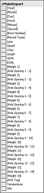
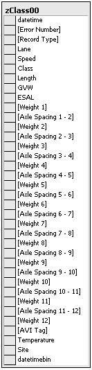
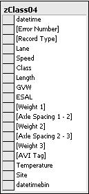
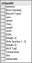
134 Additional Tables for Cube Analysis Figure 6.2 Database Schema

135 Table 6.2 WIM Database Size Table Rows Size (kb) Class ,210,337 31,704,696 Class 04 2,441, ,120 Class 05 61,835,055 4,086,744 Class 06 5,599, ,216 Class 07 1,485, ,064 Class 08 5,495, ,336 Class ,024,962 10,296,768 Class 10 1,182, ,168 Class 11 3,399, ,808 Class , ,392 Class 13 1,868, ,344 Total 382,508,246 48,194,656 Since most of the analysis performed in this research uses Class 9 trucks, a view was created that extracts data of interest from the Class 9 table and computes the left-right residual for all five axles. Views are a commonly used feature of databases that allow access to specified data in the table without using extra space to store the data. The main benefit of using a view was decreased query times. By extracting the Class 9 data records of interest from the Class 09 table, the query only examines those records instead of all records in the table Analysis Tools The final step in the data processing is the creation of a cube file. For this research, cube files were created using the Online Analytical Processing (OLAP) tools from the Microsoft SQL Analysis Server (37). Microsoft Excel can connect to the Analysis Server database and view the cube files as PivotTables and PivotCharts. It is also possible to create offline cube files for distribution that can also be viewed with Microsoft Excel. This is a convenient method of disseminating data to users that do not have online access to the database. A cube is a multi-dimensional structure that stores aggregated data and allows the data to be viewed at various detail levels (38). Figure 6.3 is provided to illustrate the analysis cube concept for this specific application. The Location axis on the main cube contains each WIM site number, allowing the user to view aggregated information for selected sites. Each Location on this axis is made up of a smaller cube that contains information for each individual lane at each WIM site, allowing the user to view aggregated information for each lane. The Time axis on the main cube contains each year of WIM data, allowing the 119

136 user to view aggregated data for the entire year. The Time axis can have many smaller cubes, depending on the level of detail. For this research, the Time dimensions are year, month, day, hour, 15- minute bin. The Measures axis on the main cube would contain the metrics that were defined in Chapters 4 and 5. The user could view the average drive tandem axle spacing, average steer axle weight, or other defined measure. View 1 illustrated in this cube could correspond to viewing the average steer axle weight for all WIM sites in January View 2 could correspond to viewing the average drive tandem axle spacing for Site 1000 for each month between January 2002 and January View 3 could correspond to viewing the average drive tandem axle spacing and average steer axle weight for Site 7340 in January There are an infinite number of views that could be used to view the data. Figure 6.3 Analysis Cube Concept The name cube suggests that these structures are three-dimensional. This is not always true. For example, a fourth dimension based on vehicle class could be added to Figure 6.3 that allowed the user to select certain vehicle classes. The metrics contained in the Measure class could also be used as extra dimensions. If steer axle weight were used as a dimension, the user could view the average drive tandem axle spacing for vehicles that had a steer axle weight within a selected range. The cube files are very powerful because they allow summary reporting using a simple structure and they allow very detailed data mining using complex structures. 120

137 The two cubes that were used for this research contain aggregated speed, axle spacing, class volume, and error count data for each individual lane. This data can be averaged and viewed for a year, month, day, hour, or 15-minute bin. Table 6.3 lists each cube, its attributes, and size. Each of these cubes contains data from January 2002 to January The Accuracy cube contains Class 9 volumes and Class 9 characteristics for analyzing the WIM accuracy. The Class Volume and Error cube contains vehicle counts for all vehicle classes except Classes 1, 2, and 3. This cube also lists errors and warnings associated with each record file. The cube manipulations are very easy to execute and the query times are usually less than a minute for updating the data. The cube is a valuable tool for examining historical WIM data from both a macroscopic and microscopic level. Table 6.3 Analysis Cube File Attributes and Size Cube Attributes Size (kb) Accuracy Cube Site Lane Date Time (15-minute bins) Class 9 volume Drive Tandem Axle Spacing Steer Axle Weight Speed 141,698 Site Lane Class Volume and Error Cube Date Time (15-minute bins) Class volumes (excluding 1, 2, 3) Errors and Warnings 435, Summary This chapter concludes the Measure step of the DMAIC performance improvement model. The data processing scheme used in this research was discussed and could be implemented by any agency. The cube file analysis will be an essential tool for agencies to begin using to view and explore WIM data. The only reporting tools that were used by INDOT prior to this research were the fixed reports produced by the WIM software. Although these reports were useful for current volume and weight data, they were not conducive to historical data exploration and data mining. The cube file analysis is much more powerful for data exploration and general trend analysis than the statistical process control charts that will be discussed in Chapter 9. The control charts are intended to use for monitoring a defined metric and making decisions for intervention, not for identifying relationships 121

138 and trends. Cube file analysis will be used in Chapter 7 for data analysis to identify trends in the accuracy metrics and the associated causes. 122

139 CHAPTER 7. DATA MINING & ROOT CAUSE ANALYSIS 7.1. Introduction The Analyze step of the DMAIC performance improvement model includes analyzing the data for trends and causes. This chapter presents a series of case studies that examine some observed trends in the drive tandem axle spacing, steer axle weight, and error rates at particular WIM sites. The error and warning types that are generated by the WIM systems in Indiana are also summarized in this chapter. For some case studies, the calibration activity log files that are stored by each WIM system were obtained and analyzed to help explain the trends. These log files are automatically generated and updated by the computer when changes are made to the sensor configuration or calibration factors. The analysis cube files that were introduced in Chapter 6 are used for the data mining and exploration. To provide an accurate representation of the data views in Microsoft Excel, minimal formatting was applied to the charts WIM Errors and Warnings WIM systems register error records whenever certain signals are generated by the sensors that are not consistent with expected signals. Other conditions related to the physics of a vehicle s speed or direction of travel can generate error records. For the equipment used In Indiana, these error records are assigned to vehicle class 0. Valid vehicle records can have warnings associated with them that indicate abnormalities with the record that did not necessarily affect the weight measurement. Table 7.1 lists the errors and warnings that are generated by the WIM systems in Indiana (36). 123

140 Table 7.1 Vendor WIM Error and Warning Description Reference Number Type Description 1 Error Axle on sensor too long 2 Error Sample queue overflow 4 Error Upstream loop only 5 Error Vehicle too fast 7 Error Downstream loop only 8 Error Upstream loop bound 9 Error Maximum axles exceeded 10 Error Zero axles detected 11 Error One axle detected 12 Error Vehicle too slow 13 Error Axle sensors in wrong order 14 Error Loops in wrong order 18 Warning Significant speed change 19 Warning Significant weight difference 20 Warning Vehicle headway too short 21 Warning Unequal axles detected 23 Warning Tailgating Certain errors are associated with sensor problems. For example, the description for error type 13 is the axle sensors are assigned in the WIM system in the wrong order. This is designed as a diagnostic error during initial site calibration or sensor replacement. However, if this error starts occurring after the system has been operational, it is attributed to a sensor threshold problem. Figure 7.1 illustrates how the piezoelectric sensor detects axles. The actual values used in the figure are not exact, but are used to illustrate the concept. The axle threshold value is programmed in the system for each sensor. When the signal exceeds that threshold, the signal is considered an axle. The strength of the signal depends on the weight of the axle. Therefore, it is possible that light axles may not be detected if the threshold value is set too high, such as threshold 1 shown in the figure. 124

141 500 Piezoelectric Sensor Output Signal Axle Threshold 1 Axle Threshold 2 Axle detected Heavy Axle (12,000 lbs) Light Axle (9,000 lbs) Baseline Signal Distance of Axle from Piezoelectric Sensor Figure 7.1 Piezoelectric Sensor Axle Detection 7.3. Case Study: Site 4200 Site 4200 is a single load cell WIM with the sensor configuration shown in Figure 4.3a. This site was known to have speed calibration problems on April 1 st, 2003 from Figure This case study will explore those problems further to identify their cause. Figure 7.2 shows a graph of the monthly average for lanes at Site The historical monthly average for lane 1 was previously shown in Figure 4.16 to illustrate the effects of speed calibration on vehicle classification. Here, the data from lane 1 is analyzed to determine potential reasons for the incorrect calibration. 125

142 6 Tandem Spacing Avg 5 Lane 1 Lane Lane 3 Site Lane January February March April May June July August September October November December January February March April May June July August September October November December January Year Month Figure 7.2 Monthly Average Drive Tandem Axle Spacing Site 4200 First, it is beneficial to determine if the change occurred gradually over time or at an exact date and time. One problem of viewing monthly and weekly averages is that the data during the intermediate month when a change was made tends to resemble a gradual change (Figure 7.2 item 1). Therefore, the daily average values for all three lanes are shown in Figure 7.3. The y-axis scale has been enlarged to provide better visualization of the data variation. The x-axis is illegible in this chart because the individual day labels are displayed. The average in lane 1 increased significantly between January 24 th and January 26 th, 2002 (Figure 7.3a). Therefore, a change was probably made on January 25 th, There were large variations in the average in lane 1 between June and August 2002 (Figure 7.3b) and between January and March 2003 (Figure 7.3c). The average decreased significantly again between August 11 th and August 13 th, 2003, so a change was probably made on August 12 th, 2003 (Figure 7.3d). 126

143 5.5 Tandem Spacing Avg Lane 1 b c 5 d 4.5 a Lane 2 Site Lane Lane January February MarchApril May June JulyAugust September October November December January February MarchApril May June JulyAugust September October November December January Year Month Day Figure 7.3 Daily Average Drive Tandem Axle Spacing Site 4200 To pinpoint when the change in January 2002 was made, the hourly average values for January 24 th, 25 th, and 26 th 2002 are shown in Figure 7.4. In this chart, the average in lane 1 clearly jumped from 4.15 feet to 5.10 feet between 13:00 and 15:00 on January 25 th. Figure 7.5 shows a portion of the calibration log file for this date. The log file confirms that the axle sensors were modified in this lane at about 14:30 on January 25 th. The number of axle sensors was increased from two to three and the calibration distance was set at 168 inches. The data for lane 3 in Figure 7.4 is not continuous because there were some hours in which no Class 9 vehicles arrived in that lane. Therefore, there was no data available for those bins to be plotted. 127

144 5.5 Tandem Spacing Avg 5 Lane Lane 2 Site Lane Lane January 2002 Year Month Day Hour Figure 7.4 Hourly Average Drive Tandem Axle Spacing Site 4200 Figure 7.5 Site 4200 Log File Excerpt The sensor that was added was a new piezoelectric sensor. The two existing axle sensors in the system were the left and right single load cell sensors. The piezoelectric axle sensor installed on January 25 th was the third installation in this lane. Figure 7.6b shows all three installation locations. A photo of the second piezoelectric sensor installation was taken on May 31 st, 2001 and is shown in Figure 7.6a. This sensor was installed downstream of the first installation. According to the log file, the second piezoelectric sensor was removed from the system on September 27 th, 2001 and had a calibration distance of 170 inches. When the third sensor was installed on January 25 th, 2002, the calibration distance should have been about 18 inches less than the distance for the second installation. However, 128

145 the calibration distance entered into the WIM system was only two inches less, making the calibration distance much longer than it should have been. This error caused the speeds and axle spacings to be overestimated. The calibration distance was either measured incorrectly or configured incorrectly causing erroneous data and unclassified vehicles. a) 2 nd Installation May 31, 2001 b) 3 rd Installation January 25 th, 2002 Figure 7.6 Site 4200 Piezoelectric Sensor Installations The calibration distance was corrected in August Figure 7.7 shows the hourly average drive tandem axle spacing for August 11 th, 12 th, and 13 th, The average decreased from 5.10 feet to 4.53 feet between 13:00 and 15:00. The log file in Figure 7.8 confirms that the calibration distance was adjusted twice at 14:30. The total distance adjustment on this date was 18 inches, or a 12% reduction, resulting in a decrease of 12.5% in the average drive tandem axle spacing. 129

146 5.5 Tandem Spacing Avg Lane Lane 2 Site Lane Lane August 2003 Year Month Day Hour Figure 7.7 Hourly Average Drive Tandem Axle Spacing Site 4200 Figure 7.8 Site 4200 Log File Excerpt Next, the large variation that was observed for lane 1 in Figure 7.3 between June and August 2002 and between January and March 2003 will be examined. First, the amount of variation in the average drive tandem axle spacing in each lane should be noted in Figure 7.3. Lane 2 exhibits the least variation, followed by lane 1, then lane 3 with the most variation. There will be less variation in the average values for lanes with high volumes and than lanes with low volumes. At site 4200, lane 1 is the right travel lane, lane 2 is the middle lane, and lane 3 is the high speed passing lane. There is an entrance ramp just upstream of the WIM sensors, so very few trucks travel in lane 1 to avoid conflicts with vehicles entering the interstate. Most of the truck traffic is located in lane 2 and the least in lane

147 Based on this information, the Class 9 volumes in lane 1 should be examined during these time periods to determine if this had an effect on the variation. Figure 7.9 shows the monthly Class 9 count distribution for all three lanes between January 2002 and January The counts in lane 1 appear to be lower in May, June, August, and September 2002 compared to those same months in However, the total counts were normal in May, June and September, indicating that the volumes shifted to lanes 2 and 3. This is likely the cause of the increased variations in lane 2. In January and February 2003, the counts in lane 1 were higher than normal, so the low volumes are not contributing to the variation in these months Class 9 Count Lane 2 Lane Site Lane Lane 1 0 January February March April May June July August September October November December January February March April May June July August September October November December January Year Month Figure 7.9 Monthly Class 9 Count Site 4200 All Lanes The long-term shifts of traffic volumes similar to that observed between May and September 2002 is usually caused by highway construction work zones and lane restrictions. The average Class 9 speeds can be examined to detect any decrease in the average speeds in all three lanes, which would likely be caused by work zones. Figure 7.10 shows the daily average speed for Class 9 vehicles in all three lanes. The average speeds decreased by approximately 4-8 mph in all three lanes between May and September 2002, supporting the presence of a work zone. According to the INDOT 2002 Annual Construction report, the interchange south of the WIM was reconstructed beginning in March 2002 and lasting for approximately seven months (39). The location of the WIM site in that work zone was near the end when 131

148 vehicles are accelerating back to normal driving speeds. Figure 7.10 also depicts the effects of the incorrect speed calibration on the speed measurement. The average speeds in lane 1 are approximately 8-10 mph higher than the speeds in lanes 2 and 3 between January 2002 and August The actual speeds were obviously not higher, but the WIM reported speeds approximately 15% too high because of the incorrect calibration. 80 Speed Avg 75 Lane Site Lane Lane 3 Lane January February MarchApril May June JulyAugust September October November December January February MarchApril May June JulyAugust September October November December January Year Month Day Figure 7.10 Daily Average Class 9 Speed Site 4200 All Lanes The variation observed in January and February 2003 is more difficult to explain. Figure 7.11 shows the hourly average drive tandem axle spacing between December 2002 and March It appears that the change in the data occurred gradually over a couple of days. There was no calibration activity reported in the site log files, so whatever caused the drift was related to the sensors or the traffic characteristics. The speeds for lane 1 shown in Figure 7.10 appear to have decreased during this time period, but they did not decrease in lane 2. Therefore, the reduction in speed is probably not related to a work zone. The work zone possibility is ruled out because it is rare that highway construction is performed during the winter months. 132

149 5.5 Tandem Spacing Avg Lane Lane 2 Site Lane Lane December January February March Year Month Day Hour Figure 7.11 Hourly Average Drive Tandem Axle Spacing Site 4200 Upon further inspection of Figure 7.3, the increased variation is also observed in January 2004 in lane 1 and lane 3. This suggests that the variation may be induced by the sensor s response to cold temperature. This site uses the left and right single load cell sensors and a single piezoelectric axle sensor to measure the speed. First, the error and warning rates in lane 1 are examined to see if they are related to the piezoelectric sensor, in particular error type 13 related to the sensor threshold. Error and warning rate charts are obtained from a different cube file that contains class volumes, errors, and warnings. Upon examination of the rates, it was discovered that the two predominant types were error 13, as expected, and warning 19, which indicates the left and right wheel weights are significantly different. Recall that warnings are assigned to record files for vehicles that are classified and have valid weights. The error record files do not have axle spacing or weight data. Figure 7.12 shows the daily count for error type 13 (black) and warning type 19 (white). Error type 13 was predominant up to January 10 th, 2003 and from February 3 rd to February 7 th, 2003 and from February 9 th to February 28 th, Warning type 19 was significant from January 15 th to January 28 th, 2003 and February 8 th to February 13 th, 2003 and February 25 th to February 26 th, It appears that when warning type 19 increases, error type 13 decreases. There is a hierarchy of errors and warnings in the WIM system because a record file cannot contain more than one error or warning code. The WIM 133

150 systems in Indiana are configured so that warning type 19 has priority over error type 13. When both of these conditions occur, only warning type 19 is reported. Therefore, the weight data is actually collected for the vehicles that generate an error, but is being discarded. The weight data could potentially be saved for this error type and possibly other error types without axle spacing data. The axle weight data is still useful for pavement design even if the vehicle classification cannot be determined. Classes All Classes 7,000 Count 6,000 5,000 4,000 3,000 Site Lane Error Number ,000 1, January February 2003 Year Month Day Figure 7.12 Site 4200 Lane 1 Error and Warning Counts Since warning type 19 is related to the wheel weights, the steer axle weight data is examined. The individual left and right wheel weight data were not archived at this site during this period, so the average total steer axle weight is used. Figure 7.13 shows the daily average drive tandem axle spacing and steer axle weight for lane 1 between December 2002 and March The steer axle weight is plotted on the secondary axis. On January 15 th, 2003, the average steer axle weight dropped to 7,000 lbs, much less than the expected average. The minimum observed average was 4,900 lbs on January 24 th, Since this weight corresponds to roughly half the average weight on a steer axle, it is assumed that only one of the wheel sensors is drifting. Also, if both sensors were drifting, the weight difference between the two would likely not be large enough to trigger a warning. On January 29 th, 2003, the average returned to 9,800 lbs without any calibration adjustments. The average weight dropped again on February 8 th, 2003 and returned to normal on February 14 th, The variations in the steer axle weight and the tandem 134

151 axle spacing appear to coincide. Therefore, the axle spacing variation is primarily attributed to a problem with one of the load cell sensors. Figure 7.13 also illustrates the importance of continuously monitoring quality control using all available data. Some agencies only monitor the data on a periodic basis, such as two weeks every month. If those two weeks were the first two weeks of the month, this sensor problem would not be detected until the first two weeks of February. However, the weight data for half of January is useless for a virtual weigh station or for planning purposes Front Axle Avg Tandem Spacing Avg Site Lane Data Tandem Spacing Avg Front Axle Avg December January February March Year Month Day Figure 7.13 Site 4200 Lane 1 Tandem Axle Spacing and Steer Axle Weight The climate data from a weather station located approximately 13 miles from the WIM station was obtained to determine the weather effects on the sensor behavior (40). Figure 7.14 shows the daily average steer axle weight and the minimum temperature obtained from the weather station. Two dotted reference lines are drawn on the graph. The upper reference line for the steer axle weight is located at 9,000 lbs. The lower reference line for the minimum temperature is located at 9 F. Whenever the minimum temperature drops below the lower reference line, the steer axle weight falls below the upper reference line. This is further emphasized with the shaded regions and is most obvious between January 15 th and January 29 th, Recall that January 15 th was the first observed date of warning type 19. This was the first day that the minimum temperature dropped below 9 F. It is hypothesized that the load 135

152 cell sensor is freezing when the temperature crosses this threshold, affecting the sensor s ability to correctly measure weights and detect axles Front Axle Avg Data Front Axle Avg Min Temp 2000 Min Temperature December January February March Year Month Day Figure 7.14 Site 4200 Lane 1 Daily Average Steer Axle Weight and Minimum Temperature This data mining case study has explored variations and discrepancies in the average drive tandem axle spacing using analysis cubes. It was shown that incorrect calibration procedures were the primary cause of the unexpected drive tandem axle spacing in lane 1 at Site Further analysis showed that variations observed in the drive tandem axle spacing were caused by both traffic characteristics and temperature. An upstream work zone affected traffic at the WIM station causing non-typical traffic patterns. The extreme cold temperatures also affected one of the single load cell sensors in lane 1. The sensor s ability to measure drive tandem axle spacing and weight accurately was severely diminished Case Study: Site 4700 Site 4700 is a piezoelectric WIM site and has the sensor configuration shown in Figure 4.3b. This site was known to have proper speed calibration on April 1 st, 2003 as verified by laser gun speed collection on this date (Figure 4.13). Therefore, data at this site was examined for variations that can arise at a site with proper calibration. Figure 7.15 shows the monthly average drive tandem axle spacing for each lane 136

153 at Site 4700 between February 2002 and January This site was reconstructed in August 2002 and sensors were added in lanes 2, 3, and 4. Therefore, the first valid data does not occur until September After September 2002, lane 1 and lane 3 appear to be the only lanes that showed much variation Tandem Spacing Avg Lane Lane Lane 4 Lane 2 Site Lane February March April May June July August September October November December January February March April May June July August September October November December January Year Month Figure 7.15 Site 4700 Monthly Average Drive Tandem Axle Spacing To determine when the variation exactly occurred, Figure 7.16 shows the daily average drive tandem axle spacing for lane 1 and lane 3 at Site The y-axis is zoomed to make the variation more noticeable. It appears that the amount of variation in both lanes increased in January It also appears that the average drive tandem axle spacing drifted in both lanes at about the same time. Both sensors exhibited much variation until August 2003, when lane 3 seemed to return to its original state right after calibration. However, in September 2003, the average in lane 1 was very erratic, suggesting a sensor problem. 137

154 4.4 Tandem Spacing Avg 4.35 Lane 1 Site Lane Lane September October November December JanuaryFebruaryMarch April May June July August September October November December January Year Month Day Figure 7.16 Site 4700 Daily Average Drive Tandem Axle Spacing The error rates in these lanes were examined for problems similar to those observed at Site The predominant error and warning in this lane were error type 13 and warning type 19. Figure 7.17 shows the monthly error count for these two errors in lane 1. It is clear that there was a large increase in errors in January 2003 that lasted until August It is interesting that the average drive tandem axle spacing became erratic in September 2003 when the error rates decreased. The two predominant error types were 13 and 19, the sensor threshold error and weight difference warning from Table 7.1. Since this site uses two piezoelectric sensors to measure axle spacing and weight, one or both of the sensors could be causing these errors. 138

155 Classes All Classes 90,000 Count 80,000 70,000 60,000 50,000 40,000 30,000 Error Number Site Lane ,000 10,000 0 September October November December January February March April May June July August September October November December Year Month Figure 7.17 Site 4700 Lane 1 Monthly Error Count Figure 7.18 shows the monthly error count in lane 3 for error type 13 and warning type 19, the two predominant types. The errors increased steadily in this lane until January 2003 and decreased afterward to the minimum in September This behavior was not consistent with lane 1, where there was an immediate spike in the error rates. Furthermore, it appears that lane 3 was experiencing a threshold problem immediately after the sensors were installed. 139

156 Classes All Classes 45,000 Count 40,000 35,000 30,000 25,000 20,000 15,000 Error Number Site Lane ,000 5,000 0 September October November December January February March April May June July August September October November December Year Month Figure 7.18 Site 4700 Lane 3 Monthly Error Count The log files were examined to determine when the thresholds were adjusted in each lane. Figure 7.19 shows an excerpt from the log file. Threshold adjustments were made to both sensors in lane 1 October 8 th, This explains the fact that error type 13 did not occur in October 2003 in Figure However, the error rates appeared to decrease in September The log files reported calibration activity on September 3 rd, The weight calibration factors were changed in lane 3 and lane 4 on this date. This suggests that adjusting the calibration factors may have an effect on the error rates or there was physical maintenance performed on the sensor on this date that reduced the error rates. There were no threshold adjustments in lane 3. Therefore, the error rate in Figure 7.18 decreased without intervention. 140

157 Figure 7.19 Site 4700 Log File Excerpt Since the error increases occurred during months with cold weather, climate data was obtained from a weather station approximately 12 miles from this WIM site. The available data at this site included the daily maximum air temperature, minimum air temperature, precipitation amount, snowfall amount, and amount of snow on the ground. Figure 7.20 shows the daily error count and daily minimum temperature for lane 1. The temperature is plotted on the secondary y-axis and the axis is reversed. Since the error rates increased over such a short amount of time, the relationship is not very clear. However, it is very likely that extreme cold temperatures contributed to the initial problem. Figure 7.21 shows the daily error count and daily minimum temperature for lane 3. There is an obvious inverse relationship between the error rates increasing and the temperature decreasing. 141

158 September October November December JanuaryFebruaryMarch April May June July August September October November December Error Count Min Temp Year Month Day Data Figure 7.20 Site 4700 Lane 1 Error Count and Minimum Temperature September October November December JanuaryFebruaryMarch April May June July August September October November December Error Count Min Temp Year Month Day Data Figure 7.21 Site 4700 Lane 3 Error Count and Minimum Temperature Min Temp Error Count Min Temp Error Count

159 The precipitation and snowfall were also examined with the error rates. Figure 7.22 shows the error rates, precipitation, and snowfall for lane 3 between March and June These months were selected because they typically experience the most rainfall and the error rates in this lane were decreasing during this time according to Figure Precipitation, in particular rain, could have an effect on the sensors if the sensors and cables are not properly sealed, allowing moisture to affect the sensor signal. According to this chart, it appears that the error rates increase during and after precipitation. It makes sense that the error rates remain for a few days after the precipitation because it takes time for the sensors to completely dry out Error Count Precipitation Data Error Rate Precipitation Snowfall Snowfall March April May June 2003 Year Month Day Figure 7.22 Site 4700 Lane 3 Error Rate and Precipitation This case study examined the drive tandem axle spacing and error rates at Site 4700, a WIM with piezoelectric sensors. There was evidence that the average drive tandem axle spacing exhibits more variation when the error rates increase. The error rates also tend to increase when the temperature decreases. When the temperature decreases, the pavement contracts and the forces on the sensor may differ from when the sensor was installed in warm weather. In lane 1, there was an immediate increase in the error rate and that error rate was sustained until maintenance was performed 9 months later. Therefore, the sensor did not recover on its own, suggesting that the sensor failed. In lane 3, the error rates increased and decreased with the temperature, suggesting that the sensor was able to recover 143

160 without intervention. There was also some evidence in this lane that the error rates may increase during and after precipitation Case Study: Site 4000 This case study will examine the weight calibration at Site 4000, the eastbound single load cell WIM on I- 80/94 that was discussed in Chapter 2. This site was constructed in January Figure 7.23 shows the monthly average steer axle weight in all four lanes at this site. The weights are all very consistent between January 2002 and April The values were all between 10,000 lbs and 11,000 lbs, indicating that the weight calibration is accurate. The average in lane 4 decreased in December 2002, but recovered the next month. In May 2003, the average in all four lanes increased Front Axle Avg Lane Lane 1 Lane 4 Lane 2 Site Lane January February March April May June July August September October November December January February March April May June July August September October November December January Year Month Figure 7.23 Site 4000 Monthly Average Steer Axle Weight First lane 4 will be examined to determine the cause of the decreased average steer axle weight in December First, the daily error rates in this lane were examined. Figure 7.24 shows the daily count of error type 19 in lane 4 between November and December Error type 19 is a warning that is triggered when the left and right wheel weights are significantly different. This error type significantly 144

161 increased on November 27 th and then decreased on December 19 th back to its normal level. The log files were examined and there was no calibration activity during this time period. Classes All Classes 300 Count Error Number Site Lane November December 2002 Year Month Day Figure 7.24 Site 4000 Lane 4 Error Type 19 Count Figure 7.25 shows the error rate and minimum temperature in this lane. The minimum temperature on November 27 th was the lowest temperature up to that time during that winter. The other peaks in the minimum temperature appear to match up with the peaks in the error rate. After December 19 th, the error rate decreased although the temperatures reached that same level again later in the month. It is hypothesized that one of the load cell sensors in this lane was freezing, similar to the load cell sensor in lane 1 at Site

162 Min Temp Data Error Rate Min Temp 50 Error Count November 2002 Year Month Day December Figure 7.25 Site 4000 Lane 4 Error Rate and Minimum Temperature Next, the shifts in the monthly steer axle weight in all four lanes that was observed in Figure 7.23 is examined. The shift occurred between April and June Figure 7.26 shows the daily average steer axle weight for all four lanes between April and June The average increased in all four lanes on May 17 th,

163 16000 Front Axle Avg Lane Lane 1 Lane 4 Lane 2 Site Lane April May June 2003 Year Month Day Figure 7.26 Site 4000 Daily Average Steer Axle Weight The log files from this site were examined for calibration activity. Figure 7.27 shows an excerpt of the log file that indicates the lanes were recalibrated on May 17 th, The calibration factors in all four lanes were modified. Prior to the recalibration, the average steer axle weights were within the expected population average. After recalibration, the averages were approximately 1,500 lbs higher than the expected population average. Therefore, the recalibration does not appear to have improved the quality of the data. 147

164 Figure 7.27 Site 4000 Log File Excerpt The error rates in all four lanes at this site were examined because this WIM site experiences more traffic than any other site in Indiana. There is a significant amount of lane changing and congestion at this site, increasing the probability of an error. For example, error types 4, 7, 10, and 14 are frequently associated with lane changing. These errors are triggered when a vehicle only activates the upstream or downstream inductive loop or when two vehicles are changing lanes and both loops are activated without activating an axle sensor. These situations occur when vehicles change lanes over the loop detectors. Figure 7.28 shows the monthly error type 13 rate and volumes for all four lanes. Error type 0 includes the record counts for Class 4 to Class 13 vehicles. These counts range from 400,000 to 600,000 each month. During July to September 2003, there are more errors generated than volumes. The predominant error type is 13 caused by the piezoelectric sensor threshold. Between January 2002 and June 2003, there was an average of 200,000 error type 13 triggers each month. Since these are errors, there is no weight data recorded for these vehicles. It is likely that a significant portion of these vehicles are passenger cars and light trucks. However, assuming that 10% of all traffic at this site is a commercial vehicle (a reasonable estimate for this facility), the weights of 700 trucks each day are not being recorded. These trucks would definitely increase the ESAL projections at this site that were presented in Chapter

165 Classes All Classes 1,200,000 Count 1,000, , ,000 Error Number Site , ,000 0 January February March April May June July August September October November December January February March April May June July August September October November December January Year Month Figure 7.28 Site 4000 Class 4-13 Volume and Error Rates The significant increase in error type 13 between July and October 2003 is examined further to determine its cause. Examination of errors on a lane basis revealed that the increase occurred in lane 2. Figure 7.29 shows the error type 13 daily count for lane 2 between July and October The error count increased significantly on July 5 th, 2003 and decreased on October 27 th, The log files reported weight recalibration activity in all four lanes on October 27 th, 2003, but nothing related to the sensor thresholds. The climate data was analyzed to explain the sudden increase in error rates. Figure 7.30 shows the daily maximum temperature and precipitation amount for July On July 5 th, 2003, a maximum temperature of 95 F was recorded. This was the maximum temperature recorded for the entire year. There was also an inch and a half of rain this day. The combination of the temperature and moisture could have adversely affected the piezoelectric sensor in this lane. Even though no threshold changes were made in October to fix the problem, physical maintenance may have been performed that fixed it. 149

166 Classes All Classes 25,000 Count 20,000 15,000 10,000 Error Number Site Lane , July August September October 2003 Year Month Day Figure 7.29 Site 4000 Lane 2 Error Type 13 Count Max Temp Data Max Temp Precipitation Precipitation July Year Month Day Figure 7.30 Site 4000 Daily Maximum Temperature and Precipitation 150

167 This case study examined the weight calibration and error rates at Site The cold temperature affected one of the single load cell sensors in lane 4 at this site. This problem was also observed in lane 1 at Site The hot temperatures and precipitation affected the piezoelectric sensor in lane 2. The error rate increased significantly in July 2003 in conjunction with the maximum temperature for 2003 and a significant amount of rainfall. The sensors at this site were incorrectly recalibrated for weight. Prior to recalibration, the average steer axle weights in all four lanes were within the expected population averages. After recalibration, the averages were too high, suggesting that the lanes should not have been recalibrated. This case study illustrates the benefits of programming site maintenance and recalibration using the procedures outlined in this report Case Study: Site 3520 This case study will examine the left-right residual and drive tandem axle spacing at Site 3520, the single load cell WIM site that was discussed in Chapter 5. The left-right residual in lanes 2 and 3 at this site were shown to have drifted, so this case study will explore reasons for that drift. Figure 7.31 shows the daily average left-right residual in all three lanes at Site 3520 between August and December The left-right residual data was only available through December 10 th, 2003 because the system was reconfigured on that date to stop logging left and right wheel data. The left-right residual in lane 1 is very erratic until November 24 th, 2003 when it drops to zero. Lane 1 is the right-most lane on a facility that has six lanes in each direction. Therefore, the truck volumes are lower than the other lanes. Lanes 2 and 3 have a more consistent left-right residual, but the slight upward trend is visible in the data. 151

168 15 Axle 1 Residual Avg 10 5 Lane Lane 1 Site Lane Lane August September October November December 2003 Year Month Day Figure 7.31 Site 3520 Daily Average Left-Right Residual To confirm that the variation in lane 1 is, in part, caused by low volumes, Figure 7.32 shows the monthly Class 9 volumes for this time period. The volumes for December 2003 are for the entire month, not just the first ten days. Lane 1 has much lower volumes than the other two lanes. However, there could be other causes for the large variations. It is very likely that one of the load cell sensors was experiencing problems because it appears that it was turned off on November 23 rd, 2003 indicated by the residual being zero. This is usually caused by the system being reconfigured so that the wheel weight from one sensor is replicated for the other sensor to obtain an estimate of the entire axle weight. Sometimes this shows up as a +100% or -100% residual. This discrepancy in reporting the data could depend on how the system is configured. Examination of the log files did not indicate that this system modification was performed on this date. Therefore, the actual cause of this sensor behavior is not clear. 152

169 Classes 9 Error Number All Error Number 40,000 Count 35,000 30,000 25,000 20,000 15,000 Site Lane ,000 5,000 0 August September October November December 2003 Year Month Figure 7.32 Site 3520 Class 9 Volumes Climate data was obtained from a weather station located approximately six miles from WIM site 3520 to examine the effects of climate on the left-right residual drift in lanes 2 and 3. The relationship in lane 3 was much more obvious than lane 2, so only lane 3 is shown in Figure The daily minimum temperature is plotted on the reversed y-axis. There is a clear relationship between the left-right residual and minimum temperature. On a macroscopic level, the overall left-right residual is increasing, or the left sensor is weighing lighter, as the temperature is decreasing. Possibly the cold temperature spikes are somehow restricting the load cell and not allowing it to compress as it is designed. 153

170 Min Temp Data Axle 1 Residual Min Temp 2 1 Axle 1 Residual August September October November December 2003 Year Month Day Figure 7.33 Site 3520 Lane 3 Daily Average Left-Right Residual and Minimum Temperature The left-right residual was also examined at this site to determine if it is accurate. Figure 7.34 shows the daily average drive tandem axle spacing in all lanes between November 2002, when the system was installed, and January There are observable cyclical variations in the data. These are attributed to the nontypical traffic on the weekends. There was a shift in the drive tandem axle spacing in all three lanes between February 5 th and February 7 th, The log files were examined to determine the cause of this shift. Figure 7.35 shows an excerpt from the log file that indicates the piezoelectric axle sensors were removed on February 6 th, Therefore, this shift is caused by the speed being measured by the inductive loop detectors after the axle sensor is removed. Since the primary and secondary speed measurement sensors have different calibration differences, the average speed shifts. However, both before and after this change, the speed calibration appears to be too high because the average values are all above 4.33 feet. 154

171 4.7 Tandem Spacing Avg Lane 2 Lane 1 Lane Site Lane November DecemberJanuaryFebruary March April May June July AugustSeptemberOctoberNovemberDecemberJanuary Year Month Day Figure 7.34 Site 3520 Daily Average Drive Tandem Axle Spacing Figure 7.35 Site 3520 Log File Excerpt It is interesting that the piezoelectric axle sensors were turned off only four months after they were installed. Figure 7.36 confirms that there was a significant amount of error type 13 up until February 2003 when the sensors were turned off. Since these errors occur with most piezoelectric sensors, perhaps the threshold adjustment should be adjusted by a temperature algorithm. There is also a significant amount 155

172 of weight data being discarded because of these errors. This error should be converted to a warning since speed and axle spacing data can still be obtained without the piezoelectric sensor. Classes All Classes 350,000 Count 300, , , ,000 Error Number Site ,000 50,000 0 November December January February March April May June July August September October November December Year Month Figure 7.36 Site 3520 Monthly Error Type 13 Counts and Class 4-13 Volumes This case study examined data from Site 3520 and showed that the drift in the left-right residual can be attributed to cold temperatures. It was previously believed that temperature did not have a significant effect on load cell sensors. However, there was evidence in this case study that it actually does. This case study also showed how switching the speed measurement from the primary to the secondary sensors can cause a shift in the average drive tandem axle spacing. The piezoelectric axle sensors at this site were all turned off within four months of the sensors being installed. This recurring problem should be addressed because it is causing much weight data to be discarded Summary The case studies presented in this chapter have identified some of the causes of certain trends in the drive tandem axle spacing, steer axle weight, left-right residual and error rates. x At Site 4200, it was observed that the speed calibration was not performed after a new piezoelectric axle sensor was installed. This caused many vehicles to not be classified 156

173 x x x because the axle spacings were overestimated. Variations in the average drive tandem axle spacing were observed in lane 1 at this site. During the summer months, the variation was attributed to speed variations caused by an upstream work zone. During the winter months, the variation was caused by problems with one of the single load cell sensors. It is hypothesized that the cold temperatures affected the load cell sensor causing speed and weight to be measured incorrectly. At Site 4700, variations in the drive tandem axle spacing were caused by piezoelectric sensor threshold problems. There was a clear relationship between the error counts increasing and the temperatures decreasing. There was also some evidence that precipitation may increase the error counts, possibly because moisture is getting into the sensor and connections. At Site 4000, a large variation in the average steer axle weight was observed in lane 4 during December It is likely that the cold temperatures affected one of the load cell sensors in that lane. The average steer axle weight in all four lanes at this site shifted out of the expected range at the same time. Examination of the log files revealed that the sensors were incorrectly recalibrated. Lane 2 at this site experienced a significant increase in piezoelectric sensor threshold errors during the summer months. These errors have been observed at other sites during the winter months and extreme cold temperatures. This lane provided evidence that they can also be caused by extreme hot temperatures. At Site 3520, the left-right residual was examined to explain the sensor drift. In lane 3, the subtle drift in the weight calibration appeared to be correlated with decreasing minimum temperatures. Also, the piezoelectric axle sensors were turned off in all three lanes at this site, forcing the inductive loops to measure speed. The shift in the average drive tandem axle spacing was observed when the change was made since the two sets of sensors had different speed calibration factors. Increased variations and average shifts are caused by non-typical traffic patterns, site maintenance, sensor modification, temperature, and precipitation. All of these factors can be accounted for except the temperature and precipitation. All of these discoveries were made using the data in the analysis cubes and climate date obtained from the internet. The WIM system is a very complex system of sensors that can be affected by numerous factors. The only way to understand these factors and how they affect the sensors is through this type of analysis. 157

174 158 CHAPTER 8. SOLUTIONS & IMPLEMENTATION 8.1. Introduction The fourth step in the DMAIC performance improvement model is to improve the processes. This improvement is accomplished by developing solutions to the problems discovered in the data analysis and implementing them. Some of the causes of poor data accuracy that were identified in the data analysis in Chapter 7 include incorrect calibration, changes in temperature, precipitation, and failing sensors. The solution to incorrect calibration is to do a better job of calibration, possibly rewriting the calibration specification and performing better enforcement of specifications. The quality control of the calibration procedures can be better assessed with the analysis cubes. The solution to the climate effects on data quality are somewhat more difficult to address, but some recommendations will be provided. This chapter will discuss a procedure for approximately tuning the calibration of a WIM system based on historical data. The results of maintenance activity for Indiana s WIM network will be presented. The accuracy metrics discussed in Chapter 4 and Chapter 5 were used to select the sites to be maintained Approximate Calibration Tuning The analysis cubes can be used to quickly generate WIM network accuracy graphs for speed and weight by examining the average drive tandem axle spacing and average steer axle weight. These graphs can be used to identify lanes that have major calibration problems and need extra attention. Site visits and calibration procedures are very expensive and can consume a significant amount of a maintenance budget. Therefore, it would be beneficial to approximately calibrate systems remotely that are grossly out of calibration. If the remote calibration is successful and the accuracy is stable, then the site can be recalibrated using the ASTM procedures when the maintenance funds become available. If the site does not maintain the calibration and the accuracy is unstable, the site likely needs further inspection and a site visit is warranted. Even if the remote calibration is not precise, this procedure can be used to get the calibration within an acceptable range until more precise calibration can be performed. For agencies that have never performed quality control of their data, this step will provide a macroscopic survey of the network accuracy level and help get it tuned.

175 Approximate Speed Calibration If the assumption that the true average Class 9 drive tandem axle spacing in a WIM lane is 4.33 feet, the speed calibration can be tuned without physically collecting individual vehicle speed data at the site. The corrected speed calibration distance can be computed using Eq. 8.1, where a is the assumed true population average 4.33 feet, a is the observed daily average drive tandem axle spacing for k recent days, d e is the current incorrect calibration distance, and d is the true calibration distance. d 1 k a k j 1 aj u d e Eq. 8.1 Since the daily average is easily obtained from the analysis cube, the average of the daily averages is used instead of the grand average of all vehicles in k days. The calibration correction should be based on ten recent days that exhibited minimal variation from non-typical traffic. In other words, do not include weekends or days that appear to have many outliers. For example, lane 2 at Site 4700 has an average drive tandem axle spacing of 4.30 feet. This lane currently has a speed calibration distance of 147 inches. The corrected distance is computed to be 148 inches. This approximate calibration procedure can be used to tune lanes that are grossly out of calibration. It will not result in a perfect speed calibration at sites where the true population average drive tandem axle spacing is not 4.33 feet. This method will also be affected by poor classification algorithms. If vehicles from other classes are mis-classified as Class 9 vehicles, the average drive tandem axle spacing will not be representative of the speed calibration. The data should be examined to make sure that there are no outliers with unreasonable drive tandem axle spacings if there is a high level of variation in the data. Using this calibration procedure can potentially save time and effort in the field collecting speed data with a laser gun. However, the laser gun is the recommended method of precisely tuning the speed calibration. Figure 8.1 shows the average drive tandem axle spacing for all lanes during May Statewide, approximately 78 out of the 156 lanes were within the individual vehicle limits of 4.25 to 4.58 feet. Only 18 of the lanes were within the expected average limits of 4.30 to 4.36 feet. The upper and lower tails of this graph are of particular interest. These lanes clearly have a calibration or sensor problem. Using this graph, individual lanes can be identified and calibration correction factors calculated to tune the speed calibration. Once the tails are eliminated from the graph, efforts can be focused on precise calibration. 159

176 8 Average Drive Tandem Axle Spacing (feet) feet = feet = 18 0 WIM Lane (n=156) Figure 8.1 Average Drive Tandem Axle Spacing All Lanes May Approximate Weight Calibration Using the left-right residual metric discussed in Chapter 5, it is probable that the weight calibration can be tuned without physically collecting vehicle data at a site. If the cross-slope of the lane is know, the upper bound value for the expected left-right residual, LRCS can be obtained from Table 5.3. A reference value for the average total steer axle weight F CG must be established based on historical data. If no other data is present, a value between 10,000 and 11,000 lbs can be selected based on the axle 1-2 spacing and Southgate s relationship shown in Figure 5.2. The expected average weights of the left wheel, F Le, and right wheel, F Re, can be calculated using Eq. 8.2 and Eq F Le F CG *( LRCS 2 1) Eq. 8.2 FRe F CG FLe Eq. 8.3 The WIM average left and right wheel weights can be obtained in a similar manner using Eq. 8.4 and Eq. 8.5, where F L is the average left wheel weight, F R is the average right wheel weight, F 1 is the average steer axle weight, and LR is the average left-right residual (decimal) for a specified number of days, k. 160

177 F L k > F 1 j * (' 1 LR k j 1 2 Eq. 8.4 F R k 1 F 1j F L k Eq. 8.5 j 1 These k days should be selected from recent data to make the calibration factors as current as possible. Days that exhibit minimal variation should be selected. However, if the process is severely out of control, the approximate calibration will only be effective for a short amount of time because the sensors are drifting. The weight calibration corrections for the left lane sensor and right lane sensor can be calculated using Eq. 8.6 and Eq W W F Le u Eq. 8.6 Lcorrected W Lcurrent F L F Re Rcorrected WRcurrent F R u Eq. 8.7 The resulting weight calibration correction will be a decimal that can be used to scale the speed calibration distance in the WIM system. For example, lane 3 at Site 3520 has an average left wheel weight of 5,667 lbs and an average right wheel weight of 5,230lbs between December 1 st and December 10 th, Assuming the average steer axle weight should be 10,300 lbs and the left-right residual caused by a -3% cross-slope is +2.8%, the expected left and right wheel weights should be 5,294 lbs and 5,005 lbs. The weight calibration factors in this lane were for both sensors. The corrected calibration factors are calculated to be and for the left and right wheel sensors, respectively. This automatic calibration procedure can be used to tune lanes that are grossly out of calibration. It will not result in a perfect weight calibration due to the variations in steer axle weight characteristics and pavement cross-slope. Using this automatic calibration procedure can potentially save time and effort in the tuning the weight calibration using a test vehicle. However, the ASTM recalibration procedure should be performed for sites that require a high level of accuracy, such as a virtual weigh station. Figure 8.2 shows the average steer axle weight for all lanes during May Approximately 72 of the 156 lanes were within the individual vehicle limits of 8,000 to 12,000 lbs. Only 53 of the lanes were within the expected population limits of 9,000 to 11,000 lbs. This graph has much bigger tails than the previous 161

178 graph. These sensors clearly have a significant calibration problem and some are not even functioning, indicated by the lower tail with no weights. The left-right residual graph should also be examined during this period to identify failed sensors. Whenever a left or right wheel sensor fails, it is common to double the weight of the functional sensor. In this case, the left-right residual would be -100% or +100% depending on the failed sensor. This is a quick method to identify failed sensors. However, since only seven sites are configured to report the left and right wheel weights, a graph of that data is not shown. 40,000 Average Steer Axle Weight (lbs) 30,000 20,000 10,000 8,000-12,000 lbs = 72 9,000-11,000 lbs = 53 0 WIM Lane (n=156) Figure 8.2 Average Steer Axle Weight All Lanes May Climate Solutions Chapter 7 showed strong evidence that temperature and precipitation affect the sensor s ability to measure speed and weight. The sensor error rates also increase in response to extreme temperature and excessive amounts of rain. It is possible that rain causes problems because moisture penetrates the sensor or cables and affects the signal. These problems could possible be minimized through better construction techniques for sealing the sensors and cable connections. Temperature variations have been known to affect the piezoelectric sensors that measure weight (29). The findings in this research provide evidence that it also affects other sensors and their functions, usually increasing error rates if a sensor is failing. 162

179 Most WIM vendor software includes an autocalibration procedure that corrects the weight calibration based on specified target values, usually based on the Class 9 steer axle weight. Temperature is collected from a temperature sensor that is installed on the paved shoulder adjacent to the sensors. The temperature is used with the Class 9 gross vehicle weight to sort the measured steer axle weights into bins. Figure 8.3 illustrates the configuration of the autocalibration bins. When a Class 9 steer axle weight is obtained, it is logged into a bin based on the temperature and the gross vehicle weight. At the end of each day, the measured steer axle weights in each bin are averaged and compared to a target steer axle weight. If these values differ by a certain percentage, then the weight calibration factors are adjusted to minimize the difference. Depending on the temperature bin size, there are many autocalibration factors considering these bins exist for each lane at the WIM site. Figure 8.3 Autocalibration Bins An evaluation of the autocalibration algorithm is recommended in future research, but for now its design and implementation do not appear to function in an acceptable manner. In Indiana, autocalibration is used for all piezoelectric sensors to account for changes in temperature. Figure 8.4 shows the daily average steer axle weight for lanes 1 and 3 at Site 4700 between January and December 2003 when autocalibration was turned on. Notice the large variations in the average values, with some of the averages falling outside of the individual vehicle weights (8,000-12,000 lbs). 163

180 Steer Axle Weight (lbs) ,000-12,000 lbs 9,000-11,000 lbs January February March April May June July August SeptemberOctober NovemberDecember Figure 8.4 Site 4700 Daily Average Steer Axle Weight (Piezoelectric Sensor) This variation is compared to the variation observed at a WIM system with single load cell sensors that do not use autocalibration. Figure 8.5 shows the daily average steer axle weight for all lanes at Site There is some variation in this data, but much less than the variations observed from the piezoelectric sensor. Furthermore, the daily averages are mostly within the expected population range (9,000-11,000 lbs). This suggests that the autocalibration algorithm could be causing the WIM system with the piezoelectric sensor to oscillate excessively. 164

181 Steer Axle Weight (lbs) 8,000-12,000 lbs 9,000-11,000 lbs January February March April May June July August SeptemberOctober NovemberDecember Figure 8.5 Site 3520 Daily Average Steer Axle Weight by Lane (Load Cell Sensor) Comparison of the average steer axle weights between single load cell and piezoelectric sensors may not be valid because single load cell sensors are deemed to be more accurate. The autocalibration algorithm was not initially enabled at Site 4700, allowing the effects of the autocalibration algorithm to be observed from a single sensor. Figure 8.6 shows the daily average steer axle weight for lane 1 at Site 4700 during April-July 2002 and April-July In 2002, the sensor was not properly calibrated, so the weights are inaccurate. It appears that there was less oscillation in the average steer axle weight in 2002 than in 2003 during the same four month period. No conclusions can be drawn from this cursory analysis, but it warrants further research to examine the autocalibration algorithm. 165

182 Steer Axle Weight (lbs) April May June July April May June July Lane 1 Figure 8.6 Site 4700 Lane 1 Daily Average Steer Axle Weight Autocalibration Comparison Instead of this step function autocalibration method, an algorithm should be developed that uses a continuous temperature value as an input. Instead of using steer axle weight for determining the factor adjustment, the left-right residual could be used so that the calibration is adjusted for each individual wheel. Weather stations should be installed at the WIM stations to measure climate data such as temperature, precipitation, and wind. This data could be incorporated into the data file to facilitate analysis. If a proper algorithm cannot be developed to account for temperature, at least the data records should be flagged indicating whether it was raining or extremely cold when the data was collected. Then, the user could make the decision as to whether the data is valid for a particular application. The data from these days would probably not be used for quality control in terms of adjusting the accuracy Implementation State agencies have limited maintenance funds for recalibrating and repairing WIM systems. There are two maintenance strategies that could be adopted for WIM system upkeep. Option #1 involves visiting all sites and performing superficial maintenance. This option provides breadth but not depth in maintenance by performing minimal maintenance on the entire network every year. Option #2 assumes complete calibration is warranted and involves thorough maintenance. This option provides depth without breadth 166

183 by performing extensive maintenance and recalibration on a few selected sites each year that are performing poorly. Prior to this research, Option #2 was not fully attainable because there was no way to determine which sites were performing poorly. Therefore, Option #1 was exercised for many years, resulting in the poor overall system health observed in Figure 8.1 and Figure 8.2. Now that WIM system performance can be ranked prior to field visits it is viable that certain sites will be targeted for extensive maintenance each year. This procedure is repeated each year until the quality of the entire WIM network is increased. Charts similar to those in Figure 8.1 and Figure 8.2 were used by INDOT in 2003 to target fourteen WIM sites for maintenance. To assess the effectiveness of this maintenance, the average drive tandem axle spacing and average steer axle weight were compared for months prior to and after the maintenance efforts. Since the maintenance occurred over a five month period, May 2003 was selected as the before month and December 2003 as the after month. Figure 8.7 shows the average drive tandem axle spacing for each lane at the fourteen targeted WIM sites. Before maintenance, in May 2003, there was 61% compliance with individual vehicle range ( feet) and 17% compliance with the expected average range ( feet). After maintenance, in December 2003, the individual vehicle range compliance increased to 88% and the expected average range increased to 50%. 7 6 May 2003 Count between ft = 40 (61%) Count between ft = 11 (17%) December 2003 Count between ft = 58 (88%) Count between ft = 33 (50%) Avg Front Axle Weight (lbs) feet feet 1 0 WIM Lane (n=66) May-03 Dec-03 Figure 8.7 Indiana Average Drive Tandem Axle Spacing for Maintained Lanes in

184 Figure 8.8 shows the average steer axle weight for each lane at the fourteen targeted WIM sites. Before maintenance, in May 2003, there was 57% compliance with individual vehicle range (8,000-12,000 lbs) and 45% compliance with the expected average range (9,000-11,000 lbs). After maintenance, in December 2003, the individual vehicle range compliance increased to 91% and the expected average range increased to 74%. 35,000 30,000 May 2003 Count between 8,000-12,000 lbs = 33 (57%) Count between 9,000-11,000 lbs = 26 (45%) December 2003 Count between 8,000-12,000 lbs = 53 (91%) Count between 9,000-11,000 lbs = 43 (74%) Avg Front Axle Weight (lbs) 25,000 20,000 15,000 10,000 8,000-12,000 lbs 9,000-11,000 lbs 5,000 0 WIM Lane (n=58) May-03 Dec-03 Figure 8.8 Indiana Average Steer Axle Weight for Maintained Lanes in 2003 Based on this data, the maintenance efforts were very effective for improving the data accuracy. These maintenance efforts could have been optimized even more because maintenance was performed on a few lanes that may not have needed extensive maintenance. After the data quality for the entire system is raised to an acceptable level, the required maintenance funds could possibly be reduced by only performing maintenance and recalibration when it is necessary Summary This chapter has presented some solutions for improving the WIM data accuracy. The speed and weight calibration factors can be approximately tuned based on historical data without conducting a site visit. This can potentially save a considerable amount of money since a site visit does not have to be made to 168

185 adjust the calibration. These procedures do not take the place of calibration, but are only used to get the calibration close enough for precise tuning on-site. Solutions need to be developed that address the climate effects on the sensor output. Possible solutions include new algorithms and installing weather stations at WIM sites to collect the required data for a new algorithm. INDOT experienced some success improving their WIM system using the accuracy graphs generated with the analysis cubes. They were able to select lanes that required calibration and see the benefits of the maintenance activity by comparing before and after accuracy metrics. 169

186 CHAPTER 9. DOCUMENTATION, PROCESS MONITORING, & POLICY CHANGES 9.1. Introduction The final step of the DMAIC model is process control. Control is accomplished through process monitoring, documentation, and policy changes. Statistical process control (SPC) is a widely used method for monitoring processes and identifying statistically significant drifts in data that warrant intervention. SPC was originally developed for use in industrial applications to monitor characteristics of widgets created in manufacturing processes. For example, a company that makes automobile cigarette lighters would be interested in monitoring the diameter of the lighters to make sure they will fit in the cigarette lighter socket being manufactured by another company. Manufacturing processes are not capable of producing identical items, so the process is monitored to make sure the widget characteristics are within defined specifications. The documentation aspect includes taking notes on all maintenance and calibration activity performed on the WIM sensors. If the site goes out of calibration and is adjusted, it should be noted for future reference. The final aspect is to invoke policy changes that will help maintain a high level of accuracy. This may involve raising the accuracy requirements for site acceptance, restructuring the calibration procedure, or invoking new site construction and maintenance policies Documentation Documentation of sensor problems, repair, and recalibration is very important for successful quality control. The calibration log files that are logged by each WIM system have been used thus far to confirm when a maintenance activity has been performed. However, these files are difficult to interpret and sometimes get erased. These files also do not contain information about physical maintenance that is performed. This type of activity is very important for quality control and explaining data trends. Each WIM system in Indiana has a book in the cabinet for technicians to write down all maintenance activity. However, this book stays in the cabinet and is only accessible by driving to the site. Historical data related to sensor installation and repair would be very useful for conducting life cycle analysis of sensors. These types of studies are not currently possible in Indiana because there is very little historical information to use. A reporting mechanism that combines these two aspects of activity logging is needed. It is not necessary for a technician to write down every single calibration factor change 170

187 when that data can be recorded by the computer. It is necessary to write down physical maintenance, site condition assessments, etc. The log files stored on the computer should be downloaded routinely and uploaded to a database for analysis. This would require restructuring of the log files to facilitate this. With the electronics available today, a laptop or personal data assistant (PDA) could be issued to all technicians to log maintenance activity. At the end of the day, the data from the PDA is uploaded to the same database. Therefore, all technicians could have access to maintenance records at all times and the historical data would be available for quality control Statistical Process Control A traffic stream is different from an industrial process because each vehicle has different characteristics. It is not expected that every vehicle will have the same speed, weight, or length. However, as shown in Chapters 4 and 5, some characteristics should be consistent for certain vehicle types. For example, the drive tandem axle spacing and the steer axle left-right residual should be constant for a population of Class 9 vehicles. Industrial SPC applications typically use subgroups of ten samples or less because it is expensive to obtain a sample. The only expense associated with traffic data is actually obtaining the data. Once the data collection system is deployed, there is virtually no marginal cost for increasing the sample size. Large sample sizes make it easier to detect true drifts in the data because the effects of outliers is reduced and the sample mean is a closer approximation of the true population mean. There have been previous applications of SPC for transportation data. The National Highway Traffic Safety Administration (NHTSA) uses control charts to assure the quality of highway crash data in their databases (41). There have been occurrences of data being coded or entered incorrectly, causing major anomalies in the data. These databases are released to the public and used for many research and evaluation applications. The public assumes this data to be accurate, so it is very important for it to be accurate. SPC is also being used for monitoring traffic data in real-time on major highways to detect incidents (42). Current hourly traffic volume, speed, and occupancy should be consistent with historical hourly data on the same day. If the data appears to be out of control, it is likely caused by an incident. SPC has been applied to the quality control of WIM data in previous research (43). That research applied SPC to the Class 9 steer axle weight. It was shown in Chapter 4 that this value varies significantly over a population of vehicles and is not precise enough to detect subtle drifts in the data. Another problem with this research was that the subgroups were formed by the first 30 vehicles each day. This sampling 171

188 procedure could cause bias in the data, considering the fact that many weight sensors are temperature dependent. The temperatures are much lower in the morning than in the middle of the day. In this chapter, SPC will be applied to the Class 9 drive tandem axle spacing, Class 9 steer axle left-right residual, and the WIM system error rates. It will be shown that SPC procedures will provide a formal process that can be used to make statistically sound decisions on when WIM speed and weight data warrant intervention Control Chart Basics Overview SPC is a formal process for identifying variation in a process that is not random. The average value and standard deviation of a process that is in control are used to establish control limits. If the process average shifts from the expected process average or the standard deviation increases, the process is said to be out of control. The shift can be attributed to an assignable cause, such as a sensor drift or failure. There are six primary steps that can be followed to determine if a process is in control. These six steps are summarized below. 1. Define subgroup frequency. 2. Define subgroup sample size. 3. Sample subgroup data from population. 4. Calculate control limits. 5. Plot control limits and subgroup averages on chart. 6. Apply defined rules to determine if process is in statistical control Subgroup Frequency The control limits are based on k subgroups of size n. A rational subgroup is a sample of items or measurements selected in a way that minimizes variation among the items or results in the sample, and maximizes the opportunity for detecting variation between the samples (44). Logical choices for subgroup frequency in this application would be an hour, day, week, or month of data. 172

189 WIM sensor drift and sensor failure usually occurs slowly over time. Data collected in consecutive hours would not be expected to vary much due to an assignable cause, such as a sensor problem. Most of the observed variation would probably be random and attributed to different vehicle characteristics. The vehicle mix at most locations changes throughout the day. For example, long-haul trucks that have certain characteristics may avoid the morning and evening rush hours, but local delivery trucks with different characteristics may not. Therefore, there would be a certain variation observed between peak hours and non-peak hours that is random. Furthermore, at low volume locations, there would be many hours during the day that did not have an adequate sample of vehicles, resulting in gaps in the control chart. For these reasons, a subgroup frequency of an hour is not ideal. A frequency of a month would likely be effective for detecting sensor drifts. However, the problem with this frequency is the lag time in obtaining a data point. For applications that require a high level of data accuracy, it is not acceptable to only check for problems once a month. This same argument could also be used for a weekly frequency. A convenient subgroup frequency is one day. Variations due to random causes are expected to be constant from day to day due to similar vehicle mixes during an entire day. Therefore observed drifts in the data are more likely attributed to the sensor. It is also possible to detect problems sooner since a data point is plotted on the control chart every day Subgroup Sample Size In terms of implementing the control charts in a database, it would be simplest to calculate averages and standard deviations for all of the vehicles during the entire day. However, the daily volumes will not be constant, especially on weekends. Most SPC applications require subgroups of equal sample size to avoid recalculation of control limits. There are SPC guidelines for using varying sample sizes, however it is not a widely used practice. Since equal samples are required for each day, the data must be sampled. In order to avoid biasing the sample, the data should be collected randomly. Random sampling was implemented for this research by sorting the Class 9 records by the seconds of the record timestamp (0 to 59 seconds). It is unlikely that this will introduce any bias in the data since the second that a vehicle arrives is a random occurrence. As opposed to obtaining a true random sample, this pseudo-random mechanism provides the user with a systematic procedure to identify the exact records that were selected in case the control chart data needs to be inspected. 173

190 Random Sampling Most data from industrial processes is normally distributed. The metrics that are used in this research are also normally distributed. SPC principles are based on properties of a normal distribution. For a given normal distribution of data, 68.26% of the data will lie within one standard deviation of the overall average, 95.44% within two standard deviations, and 99.73% within 3 standard deviations, as shown in Figure 9.1. This property is roughly the basis of the control chart limits. The data does not have to be normally distributed for SPC to be effective. It has been shown that SPC can be applied to processes with uniform distributions, right triangle distributions, Burr distributions, chi-square distributions with 2 degrees of freedom, and the exponential distribution (45). Figure 9.1 Area Under Normal Distribution Curve As stated previously, there is virtually no marginal cost to obtain an additional sample for this WIM application. The central limit theorem states that as the sample size increases, the distribution becomes more normal and the sample average gets closer to the true population average. A sample size should be chosen that is large enough to represent the true distribution of the entire sample, but small enough for a complete sample to always be available. For example, a sample size of 5,000 would not be useful in a rural location because there would never be that many trucks in a single day. A formal procedure for determining a sample size is given in Eq. 9.1, where n is the sample size, z is a statistical value 174

191 corresponding to confidence level, error (32). is the population standard deviation, and m is the desired margin of 2 z * Subgroup Sample Size n Eq. 9.1 m ¹ The z-value corresponding to 95% confidence is For this research, a single sample size of 100 was chosen for all sites because most rural sites will experience at least 100 trucks on a weekday. Eq. 9.1 will be used later to assess the margin of error based on this sample size for the SPC metrics. Rearranging the equation yields Eq z * Subgroup Margin of Error m Eq. 9.2 n Average and Standard Deviation Charts Two different types of control charts are used to monitor data, the average chart and the range chart. Subgroup averages are plotted on the average chart and subgroup ranges are plotted on the range chart. The range chart is not very robust in this application due to the existence of extreme outliers in the data set that can severely increase the range. Instead, a standard deviation chart is used that is less sensitive to outliers. To establish the control limits, the grand average and average standard deviation must be computed. Each sample is used to compute the subgroup average sample and n is the sample size. X j using Eq. 9.3, where x i is the value of the i th 1 Subgroup Average X n j x n i Eq. 9.3 i 1 The grand average X, or centerline of the control chart, is computed using Eq. 9.4, where k is the number of subgroups that the control limits are based on. 1 Grand Average X k X j Eq. 9.4 k j 1 The subgroup standard deviation s j is calculated using Eq

192 Subgroup Standard Deviation s j n (x i - X ) i 1 n-1 2 Eq. 9.5 The average standard deviation s is calculated using Eq Average Standard Deviation s k s k j Eq. 9.6 j 1 The upper and lower average control chart limits are calculated using Eq. 9.7 and Eq. 9.8, where A 3 is a constant dependent on the sample size n. Values for this constant can be obtained from Table 9.1 for a range of sample sizes up to 100. Average Upper Control Limit UCL X A s Eq. 9.7 X 3 Average Lower Control Limit LCL X A s Eq. 9.8 X 3 The constant A 3 can be approximated using Eq. 9.9 (46). A 3 3 n Eq. 9.9 Therefore, Eq. 9.7 and Eq. 9.8 can be rewritten as Eq and Eq Average Upper Control Limit UCL X X 3s n Eq Average Lower Control Limit LCL X X 3s n Eq The standard deviation control chart limits are calculated using Eq and Eq. 9.13, where B 4 and B 3 are constants dependent on the sample size n. These constants can be obtained from Table 9.1 for a range of sample sizes up to 100 (45). Standard Deviation Upper Control Limit UCL s B 4 s Eq Standard Deviation Lower Control Limit LCL s B 3 s Eq The constants B 4 and B 3 can be approximated using Eq and Eq (45). 176

193 B 4 B ( n 1) Eq ( n 1) Eq Therefore, Eq and Eq can be rewritten as Eq and Eq Standard Deviation Upper Control Limit UCL s 3 1 s 2 n 1 ( ) ¹ Eq Standard Deviation Lower Control Limit LCL s 3 1 s 2 n 1 ( ) ¹ Eq Table 9.1 Control Chart Coefficients n A 3 B 3 B Only valid and accurate data should be used to establish control chart limits. If historical data is being used to calculate the control limits, the entire data set does not have to be used. The most appropriate data to base the control limits on would be the two weeks after a site is calibrated, when it is unlikely for a calibration drift to occur. If there is a subgroup that appears to be out of control during this two week period, it should be removed and the control limits recalculated. If poor data is used to calculate the control limits, the charts will not be as effective because the limits will be inflated. 177

194 Moving Average and Moving Standard Deviation Charts The moving average is a commonly used technique for subgroups of size one to reduce the impact of a small sample size on the control limits. However, this technique can also be used for subgroups containing more than one sample to smooth the data and detect subtle drifts in the process average (47). The control limits for these charts should be tighter than the average chart and standard deviation chart to account for the increased sample sizes that are introduced by the moving average calculation. The values that are plotted on the control charts are averaged over the specified number of previous subgroups. The moving average X m and moving standard deviation s m can be calculated using Eq and Eq. 9.19, where m is the number of subgroups over which the moving average and standard deviation are calculated. 1 m m X i m i 1 Moving Average X Eq m m s i m i 1 Moving Standard Deviation s Eq The grand average and average standard deviation for the moving charts will be the same as the average chart and standard deviation chart. The upper and lower control limits for the moving average chart change to account for the increased sample sizes that are being plotted. These control limits are calculated using Eq and Eq s Upper Control Limit UCL X m X Eq n * m 3s Lower Control Limit LCL X m X Eq n * m Calculating a moving average over seven subgroups is a logical choice for this application since there are seven days in a week. This subgroup size will filter out the effects of non-typical weekend traffic where truck volumes decrease significantly on most highways. Therefore, each data point will be based on characteristics that are unique to each day of the week. Sample sizes lower than seven or higher than seven and less than fourteen could cause variations appear for some data points that include data from more than two weekends. The moving average and moving standard deviation charts are being used in this research only for visualization purposes. It will be shown that it is easier to observe the process drifting in the moving average chart because much of the daily variation gets averaged out. Theses charts should not be used to determine if the process is out of control. Since these charts are not being used for decision making, 178

195 the control limits from the average and standard deviation charts will be shown on the moving charts for consistency Plots After the control limits are established based on quality data, the subgroups are plotted on the control chart. The control limits are also plotted on the chart and should not change unless a site is recalibrated. Whenever a new subgroup is collected, the subgroup average and standard deviation are added the control chart. Figure 9.2 shows a sample average control chart with hypothetical data UCL X Subgroup Average CL X LCL X Day Figure 9.2 Sample Average Control Chart Rules After the data is plotted on the control chart, it can be tested for statistical control. There are numerous sets of SPC rules that have been developed for determining when the data in a control chart is not in statistical control. Most of the rules are primarily used for the average chart, but they can also be applied to the standard deviation chart. A run is defined as two or more points on the same side of the centerline. The rules determine the process control by assessing the length of the run and how far it is from the centerline. Many rules, require the control chart be split into six equal zones, three zones on each side of 179

196 the centerline labeled A, B, and C, as shown in Figure 9.3. Zone A is the furthest from the centerline and Zone C is the closest to the centerline. The outer boundary for Zone A is the UCL X and LCL X. The boundaries for Zone B and Zone C are computed using Eq and Eq for the average chart. 2s Zone B Boundaries X r Eq n s Zone C Boundaries X r Eq n Subgroup Average 151 UCL X CL X LCL X Zone A Zone B Zone C Zone C Zone B Zone A Day Figure 9.3 Sample Average Control Chart with Zones The first set of SPC rules were published in 1956 by the Western Electric Company (48). The rules developed by the Western Electric Company to identify a process that is not in control are listed below and illustrated in Figure 9.4 with hypothetical data. 1. A single point beyond Zone A. 2. Two out of three consecutive points in Zone A or beyond. 3. Four out of five consecutive points in Zone B or beyond. 4. Eight consecutive points in Zone C or beyond on one side of the centerline. 5. Fifteen or more consecutive points all in Zone C, above or below the centerline. 6. Eight consecutive points on both sides of the centerline, but none falling in Zone C. 180

197 7. Cyclical patterns, such as high, low, high, low. 8. A long series of consecutive points going in the same direction. Rules 1, 2, 3, and 4 are applied to one side of the centerline and rules 5, 6, 7, and 8 are applied to the entire chart. Rules 1, 2, 3, 4, and 8 indicate that the process mean has shifted. Rules 5, 6, and 7 indicate improper sampling procedures (49). Rules 7 and 8 are very subjective compared to the first six rules because they can only be tested visually or by using complex algorithms Rule UCL X Rule 3 Rule 8 Zone A 2.00 Rule 5 Zone B Subgroup Average CL X Zone C Zone C Zone B Rule 4 Rules 6,7 Zone A LCL X Rule 2 Day Figure 9.4 Western Electric Rule Illustration Nelson improved the Western Electric rules by defining run lengths for rules 7 and 8 and adjusting the run length rule 4 (50). Nelson s rules are listed below. 1. One point beyond Zone A. 2. Two out of three consecutive points in Zone A or beyond. 3. Four out of five consecutive points in Zone B or beyond. 4. Nine consecutive points in Zone C or beyond on one side of the centerline. 5. Fifteen consecutive points in Zone C above or below the centerline. 6. Eight consecutive points on both sides of the centerline with none in Zone C. 7. Fourteen consecutive points alternating up and down. 8. Six consecutive points steadily increasing or decreasing. 181

198 The probability of each of these rules being exceeded by a subgroup average can be calculated based on the area under the normal distribution curve in Figure 9.1. The subgroup averages are normally distributed according to the central limit theorem. For the first rule, the probability of one point falling outside of Zone A, or outside of 3, is 0.135%. For the second rule, the probability of two points falling beyond Zone B, or outside of 2, is ( ) 2 = 0.052%. The probabilities for all eight Western Electric rules and Nelson s rules are shown in Table 9.2. Notice that by increasing the run length for rule 4 by one, the probability of a rule violation was decreased by half. Although probabilities are still not calculated for Nelson s rules 7 and 8, the defined run length makes it much easier to apply these rules consistently. Rule Criteria Table 9.2 Probability of Rule Violations Western Electric Nelson Run Length Probability Run Length Probability 1 Outside % % 2 Outside % % 3 Outside % % 4 One Side of Centerline % % 5 Inside ± % % 6 Outside ± % % 7 Alternating Up and Down Trends There are no guidelines or defined sets of rules for given applications. The optimal rules for an application can only be obtained through experience and documentation of false calls. If the rules are too sensitive, there is a higher probability of false calls. Conversely, rules that are not sensitive enough will not detect when the process is out of control. If a process is truly out of control, most rule sets will detect this if the control limits are calculated correctly. For this research, Nelson s set of rules will be used to detect when processes are out of control Class 9 Drive Tandem Axle Spacing Characteristics In Chapter 4, it was shown that the Class 9 drive tandem axle spacing is an indicator of the speed accuracy at a WIM site. This truck characteristic is a good candidate for applying SPC procedures 182

199 because truck manufacturers only produce tandem axles with certain spacings and the population average should be fairly constant over time. The histogram in Figure 9.5 shows a histogram of the 2002 sales numbers in Table 4.1. Primarily, the spacing values are 4.25 feet and 4.33 feet. Therefore, the average drive tandem axle spacing should be near these values for a population of vehicles and should be fairly constant over time assuming the vehicle mix does not change significantly. The weighted average of the data in Table 4.1 is 4.33 feet and the standard deviation is 0.13 feet. These numbers will be used to determine the control limits. 50,000 40, Sales 30,000 20,000 10, " 52" 53" 54" 55" 56" 59" 60" Drive Tandem Axle Spacing Figure Sales Histogram The drive tandem axle spacing data was examined at Site 4700 to compare with the sales numbers. Site 4700 was shown in Figure 4.13 to have accurate speed calibration based on laser gun speeds collected on April 1, Table 9.3 and Table 9.4 show the subgroup averages, subgroup standard deviations, daily averages, daily standard deviations, and daily counts for the week following the day of data collection in lane 1 and lane 3, respectively. There is no subgroup data for lane 1 on April 4 th because there were less than 100 Class 9 trucks that day. The daily standard deviation for this day is much larger due to the lower volume of trucks. 183

200 The subgroup averages are 4.33 feet and 4.32 feet for lanes 1 and 3. This is consistent with the sales weighted average of 4.33 feet. The subgroup average standard deviations are 0.08 feet and 0.10 feet. These numbers are lower than the sales standard deviation of 0.13 feet most likely because the 4.92 and 5.00 foot spacing is underrepresented at this station. Looking at the histogram of spacings in these lanes in Figure 9.6, there were no trucks with these spacings. Although no formal tests were performed, the histogram also illustrates that the data appears to be normally distributed. Table 9.3 Site 4700 Lane 1 Drive Tandem Axle Spacing Data Day Subgroup Subgroup Daily Daily Count Average Std. Dev. Average Std. Dev. 4/1/ ,257 4/2/ ,222 4/3/ /4/ /5/ /6/ /7/ Average Table 9.4 Site 4700 Lane 3 Drive Tandem Axle Spacing Data Day Subgroup Subgroup Daily Daily Count Average Std. Dev. Average Std. Dev. 4/1/ ,666 4/2/ ,693 4/3/ ,657 4/4/ ,356 4/5/ /6/ /7/ ,410 Average

201 6,000 5,000 4,000 Frequency 3,000 2,000 1, " 50" 51" 52" 53" 54" 55" 56" 57" 58" 59" 60" Drive Tandem Axle Spacing Lane 1 Lane 3 Figure 9.6 Site 4700 Drive Tandem Axle Spacing Histogram 4/1/03-4/7/ Sample Size Recall Eq. 9.2 is used to determine the expected margin of error using a sample size of 100. The standard deviation of the sales data is 0.13 feet and the daily population standard deviation from Site 4700 lane 3 is 0.09 feet. The margin of error based on the sales standard deviation is feet at the 95% confidence level. The margin of error based on the Site 4700 data is feet at the 95% confidence level. Since most WIM systems only report the distance in feet to the nearest 0.1 feet and in inches to the nearest inch, it is not necessary to increase the sample size to obtain a margin of error that is less than the precision at which the data is reported Average and Standard Deviation Charts Control Limits The control limits for the drive tandem axle spacing can be established based on the manufacturer sales data or data from sites with accurate speed calibration. These limits should be the same for all WIM sites because speed is independent of vehicle dynamics and all WIM sites should measure identical axle 185

202 spacings for the same vehicle. From the sales data and the data from Site 4700, the grand average is assumed to be 4.33 feet. The average standard deviation is assumed to be 0.09 feet. Using these assumed values, the corresponding control limits are computed in Table 9.5. The grand average assumption could be affected by vehicle mix. It is not likely that the grand average would be higher, but it could be slightly lower, closer to the lower control limit of 4.30 feet. Consider that the WIM systems currently report distances to the nearest tenth of a foot. Therefore, if the speed were perfect, the grand average at a site with 4.25 and 4.33 foot spacings would be 4.30 feet because of the rounding. Therefore, it is suggested that histograms of the data be plotted when the process is near the lower control limit to make sure that there are indeed axle spacings less than 4.25 feet before adjusting the calibration. Table 9.5 Drive Tandem Axle Spacing Control Limits Line Equation Value (feet) Upper Zone A (UCL X ) Eq Upper Zone B Eq Upper Zone C Eq CL X Assumed from Data 4.33 Lower Zone C Eq Lower Zone B Eq Lower Zone A (LCL X ) Eq UCL s Eq CL s Assumed from Data 0.09 LCL s Eq Control Charts Data from all four lanes at Site 4700 were plotted on control charts using the proposed control limits. Figure 9.7 shows the average and standard deviation control charts for lane 1 and the Nelson rule triggers. A vertical line above or below the control limit line indicates the point that a rule violation was triggered. There were a total of 21 rule triggers in this lane. The same rule is triggered more than once in many instances. For example, rule 2 was violated on January 13 th and the next consecutive subgroup plots inside of Zone B were on January 17 th and January 18 th, At this point, the rule 2 trigger was reset. Rule 2 was violated again on January 22 nd, 2003 and was not reset until February 21 st, Even though rule 2 was violated a total of 32 days in this stretch, there were only two rule triggers. This reset procedure was followed for all of the rules. Between January and March 2003, most of the subgroup averages were below the grand average. There were many points below the lower control limit. The process exhibited a reasonable amount of control between March 2003 and September However, on September 4 th, the process average shifted and the standard deviation increased. 186

203 Average (feet) Average Legend Rule 1 Rule 2 Rule 3 Rule /01/ /15/ /29/ /12/ /26/ /12/ /26/ /09/ /23/ /07/ /21/ /04/ /18/ /02/ /16/ /30/ /13/ /27/ /10/ /24/ /08/ /22/ /05/ /19/ /03/ /17/ /31/2003 Rule 5 Rule 6 Rule 7 Rule Standard Deviation Std Dev (feet) 0.00 Figure 9.7 Site 4700 Lane 1 Average and Standard Deviation Control Chart for Drive Tandem Spacing Figure 9.8 shows the control chart for lane 2 and the Nelson rule violations. There were a total of 44 rule triggers, most of them being rule 1 outside of the lower control limit. The average data in this lane appears to be in better control than lane 1 with very little variation. However, the process average may be shifted down because the average is centered on the lower control limit. Recall that the axle spacings are only reported to the nearest tenth of a foot. Therefore, if all trucks in the sample had an axle spacing of 4.33 feet and 4.25 feet, the average would be 4.30 feet exactly because of the rounding with zero standard deviation. However, the standard deviations are greater than zero and close to the assumed standard deviation of 0.09 feet on which the control limits are based. Therefore, the calibration needs to be adjusted. 187

204 Average (feet) Average /01/ /15/ /29/ /12/ /26/ /12/ /26/2003 Standard Deviation Legend Rule 1 Rule 2 Rule 3 Rule 4 Rule 5 Rule 6 Rule 7 Rule 8 04/09/ /23/ /07/ /21/ /04/ /18/ /02/ /16/ /30/ /13/ /27/ /10/ /24/ /08/ /22/ /05/ /19/ /03/ /17/ /31/ Std Dev (feet) Figure 9.8 Site 4700 Lane 2 Average and Standard Deviation Control Chart for Drive Tandem Spacing Figure 9.9 shows the control chart for lane 3 and the Nelson rule violations. Between January and March 2003, this lane exhibited statistical control with the process average centered near the centerline. The standard deviations were outside of the control limits, but this is expected based on the inherent data variability. There were a total of 51 rule triggers and they all occurred after March In August 2003, the process average appears to have shifted down, indicated by the data points hugging the lower control limit. 188

205 Average (feet) Average Legend Rule 1 Rule 2 Rule 3 Rule 4 Rule 5 Rule 6 Rule 7 Rule Standard Deviation /01/ /15/ /29/ /12/ /26/ /12/ /26/ /09/ /23/ /07/ /21/ /04/ /18/ /02/ /16/ /30/ /13/ /27/ /10/ /24/ /08/ /22/ /05/ /19/ /03/ /17/ /31/ Std Dev (feet) Figure 9.9 Site 4700 Lane 3 Average and Standard Deviation Control Chart for Drive Tandem Spacing Figure 9.10 shows the control chart for lane 4 and Nelson rule triggers. Lane 4 is very similar to lane 2 with a process that appears to be in control with minimal variation. However, the process average is shifted down close to the lower control limit. There were a total of 42 rule triggers, but most of them were rule 1. The standard deviations in this lane are lower than the assumed average standard deviation of 0.09 feet. This suggests that the process average may actually be close to 4.30 feet. However, examination of Figure 4.13 shows that the speed accuracy was approximately 1.5% too low in this lane. Therefore, the process average needs to be shifted up. 189

206 Average (feet) Average /01/ /15/ /29/ /12/ /26/ /12/ /26/2003 Standard Deviation Legend Rule 1 Rule 2 Rule 3 Rule 4 Rule 5 Rule 6 Rule 7 Rule 8 04/09/ /23/ /07/ /21/ /04/ /18/ /02/ /16/ /30/ /13/ /27/ /10/ /24/ /08/ /22/ /05/ /19/ /03/ /17/ /31/ Std Dev (feet) Figure 9.10 Site 4700 Lane 4 Average and Standard Deviation Control Chart for Drive Tandem Spacing Based on these control charts from Site 4700, the average chart is useful for determining if the process average is accurate. The average chart also detected a shift in the process average in lane 1. However, these processes do not consistently exhibit statistical control. For that reason, it is difficult to observe the trends in the data. The next section will apply the moving average to smooth the data, making it easier to visually detect patterns Moving Average and Moving Standard Deviation The moving average and moving standard deviation charts will smooth the data, making it easier to visually observe trends in the data. The same control limits will be displayed for these charts as the average and standard deviation charts. These charts should not be used for determining the process control, but only for visualizing the data trends. Figure 9.11, Figure 9.12, Figure 9.13, and Figure 9.14 show the moving average and moving standard deviation control charts for lanes 1, 2, 3, and 4, respectively. The moving average is plotted on the primary y-axis and the moving standard deviation is plotted on the secondary y-axis. The underlying trends in the data are much more obvious in these charts than in the average and standard deviation 190

207 control charts. Early in 2003, the process mean in lane 1 appeared to be shifted down. Then, the process went completely out of control after September 5 th, The sensors in this lane should be inspected for problems. Lanes 2 and 4 need to be recalibrated to shift the process mean toward the centerline, but do not exhibit any major problems like lane 1. Lane 3 is the only lane that exhibited a process mean close to the centerline at the beginning of the chart. However, it is obvious that the process mean shifted down over time. Average (feet) Moving Average /01/ /15/ /29/ /12/ /26/ /12/ /26/ /09/ /23/ /07/ /21/ /04/ /18/ /02/ /16/ /30/ /13/ /27/ /10/ /24/ /08/ /22/ /05/ /19/ /03/ /17/ /31/ Moving Standard Deviation Std Dev (feet) 0 Figure 9.11 Site 4700 Lane 1 Moving Average and Standard Deviation for Drive Tandem Spacing 191

208 Average (feet) Moving Average /01/ /15/ /29/ /12/ /26/ /12/ /26/ /09/ /23/ /07/ /21/ /04/ /18/ /02/ /16/ /30/ /13/ /27/ /10/ /24/ /08/ /22/ /05/ /19/ /03/ /17/ /31/ Moving Standard Deviation Std Dev (feet) 0 Figure 9.12 Site 4700 Lane 2 Moving Average and Standard Deviation for Drive Tandem Spacing Average (feet) Moving Average Moving Standard Deviation 1/1/2003 1/15/2003 1/29/2003 2/12/2003 2/26/2003 3/12/2003 3/26/2003 4/9/2003 4/23/2003 5/7/2003 5/21/2003 6/4/2003 6/18/2003 7/2/2003 7/16/2003 7/30/2003 8/13/2003 8/27/2003 9/10/2003 9/24/ /8/ /22/ /5/ /19/ /3/ /17/ /31/ Std Dev (feet) Figure 9.13 Site 4700 Lane 3 Moving Average and Standard Deviation for Drive Tandem Spacing 192

209 /01/ /15/ /29/ /12/ /26/ /12/ /26/ /09/ /23/ /07/ /21/ /04/ /18/ /02/ /16/2003 Average (feet) 07/30/ /13/ /27/ /10/ /24/ /08/ /22/ /05/ /19/ /03/ /17/ /31/2003 Moving Average Moving Standard Deviation Std Dev (feet) 0 Figure 9.14 Site 4700 Lane 4 Moving Average and Standard Deviation for Drive Tandem Spacing Assignable Causes It was previously believed that the speed calibration at a site will not drift like the weight calibration. However, lanes 1 and 3 in Figure 9.11 and Figure 9.13 showed evidence of some sensor drift and data trends. Some variation that is detected may be attributed to changes in the vehicle mix. High variation may be caused by ineffective vehicle classification algorithms. It was shown in Chapter 4 that some Class 11 trucks were being classified as Class 9 trucks at a WIM site in Indiana. The spacing between the second and third axles of a Class 11 truck is around 30 feet, which would severely inflate the subgroup average and standard deviation if those vehicles are randomly selected into the subgroup. Sustained shifts in the process average are likely caused by a sensor change at the WIM system or recalibration. The speed calibration can be modified for a number of reasons. When a failing axle sensor is removed from the system, the speed is measured by the secondary sensors (inductive loops) that have a different speed calibration factor. The same thing happens when a previously failed axle sensor is replaced. The new sensor must be installed upstream or downstream of the existing sensor, changing the calibration factor. When these modifications are made, the calibration factor is not always properly adjusted. 193

210 The case study of Site 4700 in Chapter 7 showed that the drifts in lane 1 and lane 3 were due to piezoelectric sensor errors caused by temperature variations Class 9 Steer Axle Left-Right Residual Characteristics It was shown in Chapter 5 that the Class 9 steer axle left-right residual is a good metric to assess weight accuracy. This is a good characteristic for applying SPC procedures because the average value for a population of vehicles should be constant over time. Any variations in this data should be attributed to the sensor and not the vehicle mix. Depending on the cross-slope of the lane, the expected left-right residual can be obtained from Table 5.3. The monthly subgroup average and standard deviation of the left-right residual for some Indiana sites are shown in Table 9.6. For all of these lanes the average is 0.3% and the standard deviation is 6.2%. No conclusions can be drawn from this average because they have different cross-slope values. To illustrate that the left-right residual data for the entire population is normally distributed, Figure 9.15 shows the histogram for lane 2 and lane 3 at Site Although these two lanes have different population averages, it is clear that they have similar standard deviations and both appear to be normally distributed. 194

211 Table 9.6 Sample Subgroup Left-Right Residual Average and Standard Deviation Site Lane Aug-03 Sep-03 Oct-03 Nov-03 Dec-03 Total Avg Stdev Avg Stdev Avg Stdev Avg Stdev Avg Stdev Avg Stdev 1-8.4% 5.5% -9.0% 5.4% -12.9% 16.4% -6.7% 17.1% -8.7% 22.3% -9.1% 13.4% 2 4.1% 4.9% 2.9% 5.5% 3.3% 6.3% 4.2% 6.3% 3.5% 6.3% 3.6% 5.8% 3 7.3% 3.8% 7.2% 3.4% 7.3% 3.5% 6.6% 3.9% 6.6% 4.0% 7.0% 3.7% 4 0.7% 7.9% -1.0% 7.5% -1.1% 6.8% -1.4% 8.8% 1.2% 9.3% -0.4% 8.0% 1-0.8% 5.5% -1.0% 4.7% -0.9% 5.1% -1.3% 5.0% -1.0% 4.6% -1.0% 5.0% 2 2.3% 4.4% 1.7% 4.3% 1.4% 4.6% 1.9% 4.1% 1.7% 4.4% 1.8% 4.4% 2 0.3% 5.6% 0.3% 5.7% 0.4% 4.9% -0.3% 5.9% -0.1% 5.1% 0.1% 5.5% 3 1.9% 4.4% 1.4% 4.8% 1.2% 4.6% 1.6% 5.7% 1.2% 5.5% 1.5% 5.0% 1 1.3% 3.8% 0.9% 4.2% 0.7% 3.6% 0.3% 3.5% 0.4% 3.7% 0.7% 3.8% 2 0.5% 3.4% 0.9% 3.3% 1.0% 4.3% 0.7% 3.3% 1.2% 3.5% 0.9% 3.6% 1 2.8% 17.4% 2.3% 16.5% -0.4% 10.4% 3.1% 10.6% 0.1% 0.0% 1.7% 12.7% 2-8.9% 6.7% -8.5% 6.6% -8.3% 6.9% -8.0% 6.5% -7.7% 5.8% -8.3% 6.6% 3 2.0% 7.9% 2.6% 8.0% 3.6% 7.8% 3.8% 7.2% 4.1% 6.6% 3.1% 7.6% 1 8.1% 3.5% 7.5% 3.7% 8.0% 3.6% 7.5% 4.4% 8.5% 4.7% 7.9% 4.0% 2-4.3% 4.3% -4.4% 4.1% -4.7% 3.6% -4.6% 4.1% -4.8% 4.2% -4.6% 4.0% Frequency % -16% -12% -8% -4% 0% 4% 8% 12% 16% 20% Steer Axle Left-Right Residual Lane 2 Lane 3 Figure 9.15 Site 3520 Left-Right Residual Histogram 195

212 Sample Size Recall Eq. 9.2 that is used to determine the expected margin of error using a sample size of 100. The average standard deviation of the lanes in Table 9.6 is 6.2%. This standard deviation corresponds to a margin of error of 1.2% at the 95% confidence level. This margin of error corresponds to 50 pounds for a wheel that weighs 5,000 lbs. Increasing the sample size to 1,000 reduces the margin of error to 0.4%, or 20 pounds for a 5,000 lb wheel. However, this requires 10 times the amount of database storage space as a sample size of 100 and many rural sites do not experience that many Class 9 trucks in a day. Furthermore, most WIM systems only report weights to the nearest 100 lbs, so it is not necessary to increase the sample size to obtain a margin of error that is less than the precision at which the data is reported Average and Standard Deviation Charts Control Limits Each site is expected to have different control limits for this statistic. Each lane will have its own physical characteristics that affect the true average left-right residual of the population. Therefore, the control limits should be calculated using data from the first weeks after calibration, with outlying subgroups removed. Left and right wheel data was not available for any WIM sites in Indiana immediately after recalibration. Therefore, the control limits can only be calculated on data that is assumed to be accurate. Furthermore, the left and right wheel sensors are not calibrated separately in Indiana. Therefore, the magnitude of the left-right residual is not expected to match the values in Table 5.3. Even though the left and right sensors may not be calibrated correctly, SPC procedure can still detect sensor drifts. In this research, the value of the grand average will not be evaluated, only the variation of the left-right residual over time. Since the control limits will be different for each lane, data from lane 2 and lane 3 at Site 3520 is chosen for illustration. Data from August 1 st to August 14 th, 2003 was used to calculate the control limits. Table 9.7 shows the control limits for this lane. Lane 2 has a negative average left-right residual and lane 3 has a positive average left-right residual. The average standard deviation is lower in lane 2 than lane

213 Table 9.7 Left-Right Residual Control Limits for Site 3520 Lane 2 and Lane 3 Line Equation Lane 2 Lane 3 Upper Zone A (UCL X ) Eq % 4.4% Upper Zone B Eq % 3.6% Upper Zone C Eq % 2.7% CL X Eq % 1.9% Lower Zone C Eq % 1.0% Lower Zone B Eq % 0.1% Lower Zone A (LCL X ) Eq % -0.7% UCL s Eq % 10.4% CL s Eq % 8.6% LCL s Eq % 6.8% Control Charts Data from August 2003 to December 2003 for selected Indiana single load cell WIM lanes were plotted on control charts along with their estimated control limits. Figure 9.16 shows the control chart for lane 2 at Site 3520 along with the Nelson rule violations. There were a total of 18 violation triggers for rules 1 to 4. The first trigger occurred August 19 th, 2003 and the second on September 9 th, This process appeared to be in control for the first six weeks. These rules all suggest that the process mean shifted, probably caused by one of the sensors drifting. The standard deviation chart is not very useful here because most of the points are outside of the control limits. 197

214 -6% Subgroup Average 25% 22% Average -8% -10% -12% -14% Legend Rule 1 Rule 2 Rule 3 Rule 4 Rule 5 Rule 6 Rule 7 Rule 8 19% 16% 13% 10% -16% -18% 7% -20% 8/1/2003 8/8/2003 8/15/2003 8/22/2003 8/29/2003 9/5/2003 9/12/2003 9/19/2003 9/26/ /3/ /10/ /17/ /24/ /31/ /7/ /14/ /21/ /28/ /5/2003 4% Std Dev Subgroup Standard Deviation 1% Figure 9.16 Site 3520 Lane 2 Control Chart for Left-Right Residual Figure 9.17 shows the control chart for lane 3 at Site 3520 and the Nelson rule violations. There were a total of 24 violation triggers for rules 1 to 4. Again, these rules suggest that the process mean has shifted. This process appears to have been in control for the first seven weeks with only one trigger occurring on August 25 th, The subgroup standard deviation is completely outside of the control limits. In the next section the moving average and moving standard deviation charts will be applied to these sites to smooth the data. 198

215 6% Subgroup Average 27% 3% 0% -3% -6% -9% -12% -15% 8/1/2003 8/8/2003 8/15/2003 8/22/2003 8/29/2003 9/5/2003 9/12/2003 9/19/2003 9/26/ /3/ /10/ /17/ /24/ /31/ /7/ /14/ /21/ /28/ /5/2003 Average 24% 21% Legend Rule 1 Rule 2 Rule 3 Rule 4 Rule 5 Rule 6 Rule 7 Rule 8 18% 15% 12% 9% Subgroup Standard Deviation 6% 3% Std Dev Figure 9.17 Site 3520 Lane 3 Control Chart for Left-Right Residual Moving Average and Moving Standard Deviation The moving average and moving standard deviation charts are shown here to smooth the data to account for the high level of variation. The control limits for the moving average and moving standard deviation will remain the same as the average chart and standard deviation chart. These charts should only be used for trend analysis and not for determining process control. Figure 9.18 shows the moving average and moving standard deviation chart for data from lane 2 at Site The trends in the data are more evident compared to the chart in Figure It is clear that the process average in this lane has shifted. The shift is much more obvious in the moving average chart than the average chart. 199

216 -6% Moving Average 25% 22% Average -8% -10% 19% 16% -12% 13% -14% 10% -16% -18% Moving Standard Deviation 7% 4% -20% 8/1/2003 8/8/2003 8/15/2003 8/22/2003 8/29/2003 9/5/2003 9/12/2003 9/19/2003 9/26/ /3/ /10/ /17/ /24/ /31/ /7/ /14/ /21/ /28/ /5/2003 Std Dev 1% Figure 9.18 Site 3520 Lane 2 Moving Average and Standard Deviation for Left-Right Residual Figure 9.19 shows the moving average and moving standard deviation chart for data from lane 3 at Site The drift in the left-right residual in this lane is occurring much quicker than the drift in lane

217 6% Moving Average 27% 3% 0% -3% -6% -9% -12% -15% 8/1/2003 8/8/2003 8/15/2003 8/22/2003 8/29/2003 9/5/2003 9/12/2003 9/19/2003 9/26/ /3/ /10/ /17/ /24/ /31/ /7/ /14/ /21/ /28/2003 Average 12/5/ % 21% 18% 15% 12% 9% 6% Std Dev Moving Standard Deviation 3% Figure 9.19 Site 3520 Lane 3 Moving Average and Standard Deviation for Left-Right Residual Assignable Causes The weight calibration of sensors is expected to drift over time due to sensor fatigue and environmental factors such as temperature and pavement condition. Since changes in vehicle mix should not affect the left-right residual, any observed variation is likely attributed to the sensors. It was shown in the case study of Site 3520 in Figure 7.33 in Chapter 7 that the weight drift at this site can likely be attributed to the cold temperatures Error Counts This section proposes the use of proportion nonconforming charts, or p-charts, for monitoring the proportion of the error count relative to the total vehicle count each day. P-charts are referred to as attribute control charts because they are used with data that cannot be measured, but can be counted. A WIM vehicle record may or may not have an error or warning associated with it. The presence of an error or warning is an attribute of that vehicle record. 201

218 P-Charts Control Limits The error proportion is chosen opposed to the error count because the error count should be proportional to the vehicle traffic at a site. Using a proportion makes it possible to use similar control limits at all sites, regardless of the traffic. It is relatively uncommon that an error record would be generated without being initiated by a vehicle. An example when this might occur is when a sensor is chattering or turning on and off repeatedly without being triggered. However, in such a situation, the proportion of errors would be overwhelming and easily detected. Ideally, the total traffic at a site would be used to calculate the error proportion. However, most WIM systems do not log records for passenger cars and light trucks. Therefore, the records for vehicles classified as 4 to 13 and unclassified vehicles with a gross vehicle weight will be used for the total volume. Furthermore, to consider the error count as a proportion, the count of error records is included in the total volume since they are generated by vehicles. The daily error proportion p i can be calculated using Eq. 9.24, where x i is the number of error records (class 0) and n i is the total number of records (class 0, 4-13) for day i. x i p i Eq n i The average error proportion p, the centerline, is calculated using Eq. 9.25, where k is the number of days in a control period. The control period should be selected as a two week period immediately after recalibration when there should be no sensor problems. Only weekdays should be used for calculating the average error proportion since commercial vehicle traffic is significantly lower on the weekends, which tends to inflate the error proportion. CL p p i 1 k i k 1 x n i i Since the sample size n i will not be the same each day, the control limits are based on an average sample size n that is calculated using Eq The k subgroups should be the same days that were used to calculate p. Eq

219 n i k 1 k x i The standard deviation for determining the control limits is calculated using Eq Eq p ( 1 p) n Eq The upper control limit is calculated using Eq Upper Control Limit UCL p p 3 Eq In this application, there is no need to calculate a lower control limit. If the process average drops to zero, the site should be investigated because it is very unlikely that there would be no errors generated at a site. It may be desirable at some WIM sites to only use weekdays for calculating the control limits and plotting data. Since the error rate is only based on the truck traffic, the error rates tend to get inflated on the weekends when there is less truck traffic. The charts presented here do have data points plotted for the weekends, however they are not the true error rates for those weekends. The value that is plotted for Saturday is the value from the previous day, Friday, and the value that is plotted for Sunday is the value from the following day, Monday. The benefits of eliminating the values obtained for the weekends will be illustrated. Data from all four lanes at Site 4700 are used to illustrate the p-chart concept. Table 9.8 shows the p- chart control limits for all 4 lanes at Site The control limits in lane 1 and lane 2 are based on 9 weekdays in September 2002, right after the site was installed. The control limits in lane 3 and lane 4 are based on 9 weekdays in September 2003 because there was an unusually high error rate in September The centerline and upper control limit for lane 1 and lane 3 are relatively low compared to lane 2 and lane 4. At this site, lane 2 and lane 4 are the passing lanes and do not have very high volumes compared to lane 1 and lane 3. Therefore, the sample size is smaller, which inflates the control limits. 203

220 Table 9.8 Error Proportion P-Chart Limits Line Equation Lane 1 Lane 2 Lane 3 Lane 4 UCL p Eq % 23.6% 8.6% 30.7% CL p Eq % 6.8% 2.3% 11.0% Control Charts There are no rules to use with p-charts except if a data point falls above the upper control limit, action should be taken. However, some caution should be exercised if a data point above the control limit is from a weekend. The error rates on weekends can be inflated due to lower commercial vehicle traffic. Data from September 2002 to December 2003 at Site 4700 was used to illustrate the use of the p-chart. Figure 9.20, Figure 9.21, Figure 9.22, and Figure 9.23 show the p-charts for lanes 1, 2, 3, and 4, respectively, without the weekend values plotted. The dotted line is the centerline and the solid line is the upper control limit. The weekday holidays when there is non-typical truck traffic are denoted in these graphs. Many of the days that appear out of control are holidays. Lane 1 went out of control on January 6 th, 2003 and remained out of control until October 8 th, It went out of control again on November 20 th, Lane 2 appears to be in control, with the exception of two Christmas days above the upper control limit. As stated previously, lane 3 was out of control right after the site was installed in September 2002 and did not appear to be in control until August Lane 4 was also out of control right after installation and did not illustrate control until June Figure 9.24 shows the p-chart for lane 2 with the weekend values plotted. The effect of low weekend volumes is evident in this p-chart compared to Figure 9.21 depicted by large variations in the data. 204

221 50% Christmas 40% Christmas Error Proportion 30% 20% Thanksgiving 10% Thanksgiving 0% 9/1/02 10/1/02 11/1/02 12/1/02 1/1/03 2/1/03 3/1/03 4/1/03 5/1/03 6/1/03 7/1/03 8/1/03 9/1/03 10/1/03 11/1/03 12/1/03 Figure 9.20 Site 4700 Lane 1 P-Chart 50% Christmas 40% Christmas Error Proportion 30% 20% Thanksgiving Memorial Day 10% 0% 9/1/02 10/1/02 11/1/02 12/1/02 1/1/03 2/1/03 3/1/03 4/1/03 5/1/03 6/1/03 7/1/03 8/1/03 9/1/03 10/1/03 11/1/03 12/1/03 Thanksgiving Figure 9.21 Site 4700 Lane 2 P-Chart 205

222 50% Thanksgiving Christmas 40% Error Proportion 30% 20% Memorial Day Independence Day Christmas 10% Thanksgiving 0% 9/1/02 10/1/02 11/1/02 12/1/02 1/1/03 2/1/03 3/1/03 4/1/03 5/1/03 6/1/03 7/1/03 8/1/03 9/1/03 10/1/03 11/1/03 12/1/03 Figure 9.22 Site 4700 Lane 3 P-Chart 50% 40% Thanksgiving Christmas Memorial Day Thanksgiving Christmas Error Proportion 30% 20% 10% 0% 9/1/02 10/1/02 11/1/02 12/1/02 1/1/03 2/1/03 3/1/03 4/1/03 5/1/03 6/1/03 7/1/03 8/1/03 9/1/03 10/1/03 11/1/03 12/1/03 Figure 9.23 Site 4700 Lane 4 P-Chart 206

223 50% 40% 30% 20% 10% 0% 09/01/02 10/01/02 11/01/02 12/01/02 01/01/03 02/01/03 03/01/03 04/01/03 05/01/03 06/01/03 07/01/03 08/01/03 09/01/03 10/01/03 11/01/03 12/01/03 Error Proportion Figure 9.24 Site 4700 Lane 2 P-Chart Including Weekends Assignable Causes The drift in the error proportion is typically caused by sensor problems. It was shown in Chapter 7 that the error counts seem to be related to changes in temperature, particularly at this site. Other causes for out of control data points could be lower truck volumes, typical of holidays Policy Changes Policy changes should be implemented to continually improve the data quality. Examples of policy changes for this quality control program include updating construction, maintenance, and performance specifications to reflect the new procedures and solutions to known problems. For example, a new construction specification may require installing a weather station to collect temperature and precipitation measurements. The maintenance specification may require preliminary analysis of data prior to performing any recalibration, prioritizing the WIM sites and only performing maintenance on sensors that require it. The case study for Site 4000 in Chapter 7 showed that the weight calibration factors were adjusted when they did not require it. The WIM maintenance funds are very limited, so it is important that money is not wasted performing calibration when it is not needed. 207

224 Figure 9.25, Figure 9.26, and Figure 9.27 outline how the SPC charts and analysis cube files may be used for scheduling maintenance. First, the system graphs from the analysis cube file are examined for each metric (Figure 9.25a, Figure 9.26a, and Figure 9.27a). Lanes that are outside of the expected average values are identified. Then, the SPC charts for those lanes are examined to see if there is a sensor problem, calibration drift, or random noise (Figure 9.25b, Figure 9.26b, and Figure 9.27b). It is not efficient to frequently examine the SPC charts for all lanes for possible problems. It is more efficient to use the overall system graphs for possible problem identification and the SPC charts to decide if action is warranted Average Drive Tandem Axle Spacing (feet) feet Average (feet) Average Standard Deviation Std Dev (feet) WIM Lane 10/01/ /08/ /15/ /22/ /29/ /05/ /12/ /19/ /26/ /03/ /10/ /17/ /24/ /31/2003 a) System Accuracy Chart b) Statistical Process Control Chart Figure 9.25 Speed Quality Control % Subgroup Average 27% Average Front Axle Weight (lbs) ,000 to 11,000 lbs Average 3% 0% -3% -6% -9% -12% Subgroup Standard Deviation 24% 21% 18% 15% 12% 9% 6% Std Dev -15% 3% 0 WIM Lane 08/01/ /08/ /15/ /22/ /29/ /05/ /12/ /19/ /26/ /03/ /10/ /17/ /24/ /31/ /07/ /14/ /21/ /28/ /05/2003 a) System Accuracy Chart b) Statistical Process Control Chart Figure 9.26 Weight Quality Control 208

225 100% 50% 90% 80% 40% Thanksgiving Christmas Memorial Day Thanksgiving Christmas Error Rate 70% 60% 50% 40% Error Proportion 30% 20% 30% 10% 20% 10% 0% 0% WIM Lane 09/01/ /01/ /01/ /01/ /01/ /01/ /01/ /01/ /01/ /01/ /01/ /01/ /01/ /01/ /01/2003 a) System Accuracy Chart b) Statistical Process Control Chart Figure 9.27 Error Rate Quality Control 12/01/ Summary Monitoring the accuracy metrics is a crucial aspect of the DMAIC performance improvement model. SPC provides a formal evaluation procedure for discerning between noise in the data and process drift. SPC was shown in this chapter to be very effective for detecting when sensors are drifting or failing. The sample sizes and population parameters that were assumed in this chapter may not be appropriate at all WIM sites. For example, rural locations and passing lanes may never have 100 Class 9 vehicles in a day. If this is the case, the sample size can be decreased or the subgroup frequency can be decreased from one day to many days. SPC of WIM data will become a more effective tool as agencies gain experience using the control charts. This will facilitate better understanding of patterns in the data and how sensors behave prior to failure, leading to more effective quality control. 209

226 210 CHAPTER 10. CONCLUSIONS Summary This report has outlined the DMAIC performance improvement model that is commonly used for Six Sigma quality control programs. Each step of the model was addressed and applied to the WIM data quality, providing a solid framework for agencies to implement this procedure for their own WIM network. Chapter 2 defined the motivation and problem statement for improving the WIM data accuracy. Analysis of WIM data in northwest Indiana suggested that there is a significant problem with trucks hauling overweight. Overweight trucks significantly decrease the pavement life. Therefore, it is important to identify overweight trucks to deter them from hauling overweight in the future. Most weight enforcement is currently conducted at static weigh stations and some occasional mobile enforcement. The static weigh station study conducted with ISP provided evidence that static weigh stations are not effective for identifying overweight trucks. Limited tests showed that virtual weigh stations in Indiana are approximately 55 times more effective than static weigh stations for identifying overweight trucks. The virtual weigh stations use existing WIM sensors to allow enforcement officer to view weight data in realtime to screen trucks on the highway for overweight violations. The primary limitation to widespread virtual weigh station deployment is the WIM data quality. This proposed quality control program documented in this report will help ensure accurate and reliable WIM data to support virtual weigh stations. Chapter 3 outlined the ASTM WIM standard specification. This specification defines calibration and acceptance testing procedures for various WIM applications. These procedures are based on tuning the WIM system calibration so that the dynamic weights are close to the static weights. This testing procedure is very tedious to conduct and the accuracy requirements are difficult to enforce. Using the metrics identified in Chapter 4 and Chapter 5, the system accuracy can be more effectively monitored continuously by comparing the metric values to population averages. Chapter 4 identified the speed and axle spacing accuracy metric. Accurate speeds are required to calculate the correct axle spacing. Accurate axle spacing data is required to properly classify vehicles. It was shown in Chapter 4 that incorrect speed calibration and axle spacing estimates can cause vehicles to

227 be misclassified or not classified at all. The WIM axle spacing is calculated from the WIM measured speed, so a single metric will used to assess the accuracy of both. The drive tandem axle spacing for Class 9 trucks is a consistent value because manufacturers only produce trucks with certain axle spacing distances. The lower and upper bound values for individual trucks are 4.25 feet and 4.58 feet. The lower and upper bound values for the expected population average are 4.30 feet and 4.36 feet. The relationship between the speed accuracy and the expected drive tandem axle spacing value was validated at selected WIM sites in Indiana using a laser speed gun to collect the true vehicle weights. This metric can be calculated for all WIM lanes in the system to quickly assess the data accuracy. Chapter 5 identified the weight accuracy metric. Previous research showed that the steer axle weight for Class 9 trucks should be between 8,000 lbs and 12,000 lbs for individual vehicles. Based on data analysis in Indiana, the population average should be between 9,000 lbs and 11,000 lbs. Although these values are useful for approximately assessing the weight accuracy, the steer axle weight is not robust enough to detect a subtle calibration drift. A new metric, the left-right residual, calculates the difference between the left wheel and right wheel on the Class 9 steer axle. The distribution of weight on the steer axle should be equal between the left and right wheels, yielding a residual close to zero. The residual is affected by the roadway cross-slope, but correction factors are provided. The left-right residual can only be calculated for WIM systems that measure wheel weights, such as load cell or bending plate systems. A residual can also be calculated for WIM systems that have sequentially redundant sensors that only measure total axle weights, such as piezoelectric or other strip sensor systems. The left-right residual was shown to be very effective for detecting slight drifts in WIM weight sensor calibration. Using the steer axle left-right residual in conjunction with the total steer axle weight allows the drifting sensor to be identified without physically testing the sensor. This could prevent having to replace or adjust sensors that are functioning properly. Chapter 6 outlined the WIM data processing procedure employed for this research. Many agencies only analyze WIM data using the vendor software that only generates fixed reports for individual sites. To apply the quality control procedures outlined in this research, the raw vehicle records must be uploaded to a relational database that supports free-form queries. Another tool that was applied for data mining was analysis cubes. Analysis cubes provide a mechanism for aggregating data so that it is easily viewed in table or chart format. The cubes allow views of data at various levels of time detail. The analysis cubes for this research contained site and lane data for two years of WIM data. The measures that were aggregated were vehicle count, axle weights, axle spacing, gross vehicle weights, speeds, and error rates. 211

228 Chapter 7 presented case studies that analyzed trends in the WIM data in Indiana. The data mining was performed using the analysis cubes to explore unexpected data variations in the accuracy metrics. Some of the problems that were identified were incorrect calibration, sensor failure, and sensor drift. The sensor failure and sensor drift in some cases was shown to be related to extreme temperatures and precipitation. Climate data was obtained from weather stations in close proximity to the WIM sites to explore potential relationships. The weather effects were a significant finding because it was previously believed that temperature only affected the weight measurement by piezoelectric sensors, and temperature could effectively be compensated for. Chapter 8 discussed strategies for improving the accuracy. Approximate calibration correction factors can be calculated for the speed and weight accuracy based on the expected population averages and the observed averages. These procedures can be used at the outset of a quality control program to approximately calibrate the system. Performing approximate calibration can potentially save money required to conduct the ASTM calibration procedure that involves driving test vehicles over the sensors. This chapter also presents the results of a study that examined the effectiveness of WIM maintenance activity in 2003 in Indiana. Accuracy plots using the metrics identified in Chapter 4 and Chapter 5 were used to focus maintenance funds on WIM sites that were incorrectly calibrated. Analysis of data before and after the maintenance activity showed an increase in the number of lanes that were compliant with the expected population averages. The approximate annual maintenance budget for INDOT is $400,000 per year. Considering there are approximately 156 WIM lanes in Indiana s network, there is approximately $2,500 per lane per year for maintenance. According to one vendor s estimates, the annual maintenance costs for a WIM lane is $4,800 per year (51). Therefore, it is very important to prioritize the maintenance. Chapter 9 discussed the statistical process control procedure that is used for monitoring the accuracy metrics over time. Statistical process control provides a mechanism for determining when observed variations can be attributed to sensor problems and not random noise in the data so that decisions can be made to intervene and repair or recalibrate sensors. Recalibration and maintenance is usually performed at set intervals regardless of whether the sensor requires attention. Using the SPC procedure, the maintenance can be prioritized to most effectively allocate scarce maintenance funds. This chapter also stressed the importance of documenting sensor maintenance, recalibration, and observed data trends to gain more insight into sensor behavior over time. 212

229 10.2. Contributions The major contribution of this report to the WIM vendors is the development of sound analysis procedures that show the WIM systems in Indiana are not in statistical control. There are factors, particularly temperature and precipitation, which are not being properly accounted for in the signal processing algorithms. A high level of accuracy and reliability cannot be obtained until these factors are incorporated into the WIM system algorithms using climate data obtained from weather stations that need to be installed at each WIM location. The major contribution of this report to WIM users, particularly state agencies, is a set of tools that can be used to assess the data accuracy and monitor it over time. Identification of the accuracy metrics to use in this procedure was very important. The Class 9 drive tandem axle spacing was identified for monitoring speed and axle spacing accuracy. The Class 9 left-right residual was defined for monitoring weight accuracy. Using the tools developed in this research, maintenance funds can be prioritized so it is only performed on the sensors that require maintenance or recalibration when there is a problem detected using by the statistical process control charts Recommendations Based on experiences in this research and the information summarized in this report, recommendations were made to address the WIM system configuration, vendor software, and standard specification. Implementation of the system configuration recommendations will provide higher quality data from the WIM system. The vendor software modifications will simplify the efforts required to process the data for analysis. The WIM standard modifications address some of the perceived shortcomings of the current ASTM standard WIM System Modifications It was hypothesized based on the data analysis in Chapter 7 that there is a significant amount of weight data that is being discarded because of certain error types. Error type 13 is generated by piezoelectric axle sensors when there is a threshold problem, usually caused by temperature changes. At sites where piezoelectric sensors are only used for speed and axle spacing, the speed data can also be obtained with the inductive loop detectors. The load cell or bending plate sensors obtain the weights and can measure the time between consecutive axles. This operation is already performed when the piezoelectric sensor is turned off. The only system modification that would have to be made is for the inductive loops to also collect speed for every vehicle and change error type 13 to a warning. When this warning is triggered, 213

230 the inductive loop speed is used to calculate the axle spacings instead of the system trying to use the speed from the axle sensors. Another cause of variation in the drive tandem axle spacing was vehicle acceleration. Variations were observed at Site 4200 because of a work zone and vehicles were changing speed. When the axle sensors are being used to measure speed, it can be measured for each individual axle. The speed based on the first axle can be compared to the speed based on the last axle to determine if the vehicle is traveling at a constant speed. If the vehicle is accelerating or decelerating, a warning code should be indicated in that record file so that data is not used for quality control or accuracy checks. ASTM WIM types III and IV are currently required to determine if a vehicle is accelerating or decelerating. Those systems may already determine this in a similar manner to what was described here. Since the WIM systems used for virtual weigh stations are type II data collection sites, they are not required to identify acceleration. Another modification related to speed is the precision at which it is reported. Currently, WIM systems are only required by the ASTM specification to collect axle spacing data to the nearest tenth of a foot. This makes interpretation of control charts very difficult because two of the common spacings both round to 4.30 feet. The axle spacing should be reported to hundredths of a foot, allowing the precise axle spacing to be obtained and binned in the proper category. This modification will improve the grand average and standard deviation estimates calculated in Table 9.5. The data records produced by WIM systems in Indiana only contain one column for reporting errors and warnings. Therefore, if a vehicle triggers more than one, the error or warning with the highest programmed priority gets reported. This procedure is not effective for quality control and understanding data trends. One solution would be to have multiple columns for reporting errors and warnings, however this would be difficult to manage in a database. Another solution may be to report errors and warnings in a record file separate from the resulting vehicle data file. Association of warnings and errors with the vehicle data file can be performed by matching the timestamp and the lane number. The vehicle classification file should be optimized to reflect the vehicle types traveling in the area. For example, it was shown in Chapter 4 that some Class 11 vehicles were being assigned to Class 9. This was partially caused by incorrect speed calibration, but would have never occurred if the classification file were better tuned. Many state agencies use the vendor default classification file, which probably does not apply to every state. Another modification to the classification file is the handling of unclassified vehicles. The error record files should remain as Class 0 vehicles. However, unclassifiable vehicles based on unconventional axle configurations should be assigned to Class 14. These vehicles are not 214

231 errors and should not be treated as such. Quite often, the weights of these unclassifiable vehicles are not accounted for in pavement design and evaluation because the user does not know they are there. Often, these are the heaviest vehicles on the roadway because they have special axle configurations to be allowed to haul extremely heavy loads. Calibration and maintenance records must be incorporated into the data transfer procedure so that a historical record of activity is available at any time. First, this would require reformatting the current log files to be conducive to a database structure. Next, the system should be compatible with a PDA to transfer maintenance logs kept by the technician. Historical maintenance and calibration records are vital to understanding sensor behavior. Solutions need to be developed to address the effects of climate on the sensors. Chapter 7 provided evidence that extreme temperatures and precipitation can cause error rates to increase and calibration to drift. The current autocalibration feature is not robust enough to account for this. The first step is to install weather stations at selected WIM site to collect accurate temperature and precipitation data. Once this data is available to the WIM system, new algorithms must be developed that use this new information. If the algorithms are not successful, the vehicle record file should reflect the temperatures and existence of precipitation so the end user can make decisions on whether to use the data for a particular application WIM Standard Modifications The ASTM WIM standard should be modified to include a new category of WIM type that combines the accuracy requirements of Type III with the data requirements of Type II. Virtual weigh stations use WIM sensors that are primarily used for data collection. Type II systems are intended for data collection purposes and have looser accuracy thresholds than Type III that are used for enforcement. However, Type III systems are not required to classify vehicles or estimate ESAL. This information is very important for data collection and possibly enforcement. It is helpful for the officer using the virtual weigh station to know what type of truck is violating to help identify it in the traffic stream. The ASTM accuracy tolerances for speed and axle spacing should also be rewritten. From Table 3.3, the ASTM WIM standard accuracy tolerances for speed and axle spacing were ±1 mph and ±0.5 feet. Based on the relationships in Eq. 4.3 and Eq. 4.4, the speed and axle spacing data reported by the WIM are directly related. The percentage error in the calibration distance will result in the same error in the speed and axle spacing measurements. Therefore, the tolerances for these measurements should reflect this relationship. The tolerances in Table 3.3 are independent of the vehicle speed because the acceptance 215

232 test can be performed at speeds ranging from 10 mph to 80 mph, yet the same tolerances are used for both speeds. At 10 mph, a difference of 1 mph allows a 10% error in the speed measurement. At 80 mph, a difference of 1 mph only allows a 1.25% error in the speed measurement. Assume a WIM system has a speed calibration error of -5%. At 80 mph, the measured speed would be 76 mph resulting in the WIM not being in compliance. However, at 10 mph, the measured speed would be 9.5 mph resulting in the WIM being in compliance. This inconsistency could cause confusion during acceptance testing and also presents a loophole that could be exploited to get a non-compliant WIM system accepted. The same problem exists for the axle spacing. The standard does not specify a particular axle spacing measurement to apply the tolerance. Consider the axle spacing distances for a Class 9 truck, one of the test vehicles. The typical spacing between axle 2 and 3 is 4.3 feet. The typical spacing between axle 3 and 4 is feet. The tolerance of 0.5 feet allows an error of 12% for the spacing between axle 2 and 3 and an error of 1.7% for the spacing between axle 3 and 4. Similar to the speed, this tolerance will not produce consistent results for all axle spacing distances. The speed and axle spacing tolerances should be specified as percentages, similar to the weight tolerances. Both of these measurements are going to reflect the error in the speed calibration. This modification will provide consistent testing results and eliminate the probability of a non-conforming system to be accepted. The weight accuracy thresholds should also be assessed. From Table 3.3, the wheel, axle, and gross vehicle weight accuracy thresholds are ±20%, ±15%, and ±6%, respectively. It is believed that these graduated criteria originated due to the load shifting that occurs while a vehicle is moving. WIM vendors state that the wheel and axle accuracy is hard to achieve, but the gross vehicle weight is not. The problem with these criteria is the fact that wheel and axle loads can be off by as much as 20%. This may not be a significant problem for enforcement purposes because most mobile enforcement is targeted toward gross vehicle weight violations. This is a significant problem for pavement design and evaluation. Recall that the ESAL calculation is based on individual and tandem axle weights, not gross vehicle weights. A 20% error in these axle weights will significantly skew the ESAL calculations, resulting in poor design and evaluation. This will be especially important for the 2002 Pavement Design Guide that will develop new pavement design models based on these data. The final WIM standard modification is to incorporate the accuracy metrics identified in this report. The drive tandem axle spacing and left-right residual are clear indicators of speed and weight accuracy. They are much easier to test and monitor than the current accuracy requirements based on comparison of static vehicle weights with dynamic vehicle weights. A new performance-based specification could be 216

233 used to evaluate long-term WIM performance, something that is currently done by very few agencies. These performance criteria could be incorporated into a construction or maintenance contract, similar to some pavement installation specifications Future Research Most of the future research that stems from this report is related to sensor evaluation and understanding of factors that affect their performance. There have been few comprehensive studies that compare and contrast all WIM sensor types, their expected life, maintenance frequency, and sustained accuracy. If multiple sensor types were all installed in the same segment of pavement so that they all received the same loading, environment, pavement smoothness, and pavement composition, valid comparisons could be made between each sensor type. This type of information would be extremely useful to many agencies for selecting a certain sensor type to suit its application. Strip sensors may be less expensive and less accurate than load cell sensors, but there are certain applications where they would be very useful. For example, if there is a bypass route that experiences heavy trucks, as soon as enforcement is conducted at that location for a few months, the overweight trucks will stop using that highway and the sensors will not be used any more. However, on an extremely congested interstate, it may be more longterm cost effective to use the most expensive sensor with the longest service life to minimize the number and duration of road closures for maintenance and replacement. This type of study could be conducted using a sensor installation similar to the one shown in Figure This hypothetical layout would test three different strip sensors and two load cell sensors. A test site should be constructed in asphalt and another test site in Portland cement concrete. The asphalt test might not include the load cell sensors because they require a concrete vault and a very firm foundation. The factors that would be examined include response to climate, weight accuracy, speed accuracy, accuracy longevity, failure rates, and maintenance frequency, among others. Ideally, the site would be constructed upstream of a static weigh station. Therefore, static weights of vehicles could easily be obtained for comparing the WIM weights. 217

234 Figure 10.1 Redundant Sensor Testing Layout The WIM system with redundant sensors will also provide a good mechanism for evaluating the autocalibration algorithms that are used by many WIM vendors for adjusting weight calibration for temperature variation. The piezoelectric sensor was shown in this research to be affected by extreme temperatures. Although the load cell was also affected, it did not experience the high error rates that the piezoelectric sensor did. Therefore, the autocalibration algorithm for the piezoelectric sensors can be evaluated to determine its usefulness and identify possible improvements. Another important weight accuracy aspect that shall be examined is the lateral location of the wheel on the sensor. WIM sensors should be capable of weighing a wheel load accurately whether it is located in the center of the sensor or near the edge. The ASTM WIM specification states that the wheel weight 218

235 measurement cannot vary by more than 2% across the width of the sensor. This requirement is rarely tested. However, this sensor layout provides a mechanism for evaluating this specification for all sensor types. The static weights could be obtained from the downstream static weigh station. The final weight accuracy issue that is very important for pavement design is each sensor s ability to measure heavy axle loads. Consider the vehicle that had a static gross vehicle weight of 120,000 lbs in Figure 1.6. The WIM weight was 10,000 lbs too light. Heavy axle loads do the most damage to the roadway. Therefore, it is important to accurate measure these loads for pavement design and evaluation. It is very difficult to determine the accuracy at which a sensor measures these heavy loads. The accuracy cannot be determined using a test vehicle because the vehicle should not violate any weight laws. Furthermore, it is not desirable to exert excessive damage to the pavement for testing purposes. There is an opportunity to determine the accuracy from permitted loads. Trucking companies can purchase special permits for hauling overweight. This is typically done when a heavy item cannot be divided into smaller legal loads. Many of these extreme loads are issued a police escort through the state to ensure the vehicle does not travel on any unauthorized highways and for the safety of other vehicles. Therefore, the date and time that these heavy vehicles will cross the sensors can be approximated. These vehicles are usually statically weighed at a weigh station to make sure they do not weigh more than they are permitted to weigh. Therefore, the static weights could be obtained from police records. Even though this method is tedious and would take a long time to acquire a large dataset, it is the most feasible option for collecting this type of data. A second study would evaluate specific sensor behavior with respect to construction techniques, pavement material, pavement smoothness, geographic location, and traffic loading. All of these factors should affect sensor performance and service life. Some aspects of this study could be accomplished with current in-service WIM systems. However, new installations would also be required to document various construction techniques. The WIM systems that were installed under the LTPP program should cover a wide range of these factors because they are monitoring pavements that were specifically selected per these criteria. The main limitation to using this plan is obtaining historical data. Indiana has been active with the LTPP program, but has minimal documentation of installation and maintenance activity and the WIM systems are not accurate. This is likely the situation for many other states involved in the LTPP program. One last future research project will examine the effects of pavement smoothness on weight measurements. It is known that rough pavement will increase vehicle dynamics and decrease the weight accuracy. For a virtual weigh station, this is very undesirable because the weight estimates are very unpredictable depending if the weight is measured on the upbounce or downbounce. If the pavement is 219

236 smooth and the calibration is too high or too low, the enforcement officer can get a feel for the error and compensate for it when identifying overweight trucks. This cannot be done when the weight errors are random. It is hypothesized that the pavement smoothness in a WIM lane can be evaluated by calculating the residual of the drive tandem axle weights. Based on data obtained from static weigh stations in Indiana, the lead drive tandem axle should weigh approximately 250 lbs more than the second drive tandem axle. The weight difference is attributed to the lead axle being the main drive axle with the drive assembly attached to it. If the average drive tandem residual in a lane is not close to 250 lbs, then the lane is possibly unsmooth. This metric would be useful for identifying existing WIM stations to be used for virtual weigh stations. 220

237 221 LIST OF REFERENCES (1) Riverson, J. and Sinha, K. (1988). Evaluation of the Coordination of Weigh-in-Motion Truck Data in Indiana. Joint Highway Research Program Report No. FHWA/IN/JHRP-88/7. Department of Civil Engineering, Purdue University, West Lafayette, Indiana. (2) Welcome to LTPP. (2003). Long-Term Pavement Performance program. Federal Highway Administration. April < (3) PowerPoint Presentation : Overview of LTPP Program. Long-Term Pavement Performance program. Federal Highway Administration. April < (4) LTPP Traffic QC Software, Volume 1: Users Guide. Software version 1.6. November (5) Green, J., Nichols, A., Allen, E., Nuber, L., Thomaz, J., Bullock, D., and Wasson, J. (2002). Virtual Weigh Station. Joint Transportation Research Program Report No. FHWA/IN/JTRP-2001/09. Department of Civil Engineering, Purdue University, West Lafayette, Indiana. (6) Hanson, M. (2004). Roadway sensors replacing state's weigh stations. The Bismarck Tribune, Bismarck, N.D. (7) Nichols, A., Bullock, D., Boruff, G., Newland, M., and Wasson, J. (2002). Enforcement Procedures Using Weigh-in-Motion Systems in Indiana. Proceedings from the 9th World Congress on Intelligent Transportation Systems, Chicago, Il. (8) Kruker, M. and Evert, K. (1992). Mainline Screening for Enforcement. Paper presented at National Traffic Data Acquisition Conference, Sacramento, CA, October (9) Slevin, J. (1999). PrePass and NORPASS. ITS World, Volume 4, Number 3, pp (10) Ruback, L. and Middleton, D. (1999) Demonstration of a Mobile Application of CVO Weight Enforcement Screening. Report No. TTI/ITS RCE-99/03. Texas Transportation Institute, College Station, Texas. (11) AASHTO 2002 Pavement Design Guide. Developed under NCHRP Project 1-37A, under contract with ERES Consultants, Inc. (12) LTPP and the 2002 Pavement Design Guide Brochure. (2003) Report No. FHWA-RD (13) Pyzdek, T. (1999). The Complete Guide to Six Sigma. Quality Publishing. (14) National Institute of Standards and Technology (NIST). Press release obtained from website. April < (15) Pyzdek, T. (2001). The Six Sigma Handbook. McGraw-Hill, New York.

238 (16) Stamatis, D. (2002). Six Sigma and Beyond, Volume 1. St. Lucie Press. (17) Federal Highway Administration (FHWA). (1992). Traffic Monitoring Guide. Publication No. FHWA- PL , Washington D.C. (18) AASHTO Guide for Design of Pavement Structures. (1993). The American Association of State Highway and Transportation Officials, Washington, D.C. (19) from Kumar Dave September 16, INDOT Pavement Design Engineer. (20) Indiana Department of Transportation. (1971). Indiana Pavement Design Manual, Chapter 52. (21) Mannering, F. (1993). Male/female driver characteristics and accident risk: some new evidence. Accident Analysis and Prevention 25, pp (22) Mannering, F. and Hamed, M. (1990). Occurrence, frequency, and duration of commuters work-tohome departure delay. Transportation Research 24B, pp (23) Washington, S., Karlaftis, M., and Mannering, F. (2003). Statistical and Econometric Methods for Transportation Data Analysis. Chapman and Hall Publishing. (24) Nam, D. and Mannering, F. (2000). Hazard-based analysis of highway incident duration. Transportation Research 34A, pp (25) American Society for Testing and Materials (ASTM). (2002). E : Standard Specification for Highway Weigh-in-Motion (WIM) Systems with User Requirements and Test Method. ASTM Committee E-17 on Vehicle-Pavement Systems. (26) Mondal, A., Hand, A., and Ward, D. (2000). Evaluation of Lightweight Non-Contact Profilers. Joint Transportation Research Program Report No. FHWA/IN/JTRP-2000/06. Department of Civil Engineering, Purdue University, West Lafayette, Indiana. (27) Long Term Pavement Performance Project, TDP-18. (2001) Guide to LTPP Traffic Data Collection and Processing. Federal Highway Administration, U.S. Department of Transportation. (28) Long Term Pavement Performance Project. (2000). Draft: Verification of Accuracy of LTPP SPS WIM Sites. Federal Highway Administration, U.S. Department of Transportation. (29) McCall B. and Vodrazka, W. (1997). States Successful Practices Weigh-in-Motion Handbook. Federal Highway Administration. (30) Society of Automotive Engineers. (1985). J683: Tire Chain Clearance. SAE Information Report. (31) International Road Dynamics, Inc. (2001). Weigh-in-Motion Technology Comparisons. Technical Brief obtained from website. April < (32) Moore, D. and McCabe, G. (1999). Introduction to the Practice of Statistics, 3rd Edition. W.H. Freeman and Company, New York. (33) Dahlin, C. (1992). Proposed Method for Calibrating Weigh-in-Motion Systems and for Monitoring that Calibration Over Time. Transportation Research Record 1364, TRB, National Research Council, Washington D.C., pp

239 (34) Southgate, H. Quality Assurance of Weigh-in-Motion Data. Undated white paper on Federal Highway Administration website, FHWA Contract No. DTFH61-P (35) Izadmehr, B. and Lee, C. (1987). On-Site Calibration of Weigh-in-Motion Systems. Transportation Research Record 1123, TRB, National Research Council, Washington D.C., pp (36) International Road Dynamics Inc. (IRD). (1999) IRD Weigh-in-Motion Data Collection System Software Users Manual, V Saskatoon, Saskatchewan. (37) Jacobson, R. (2000). SQL Server 2000 Analysis Services. Microsoft Press, Redmond, Washington. (38) Seidman, C. (2001). Data Mining with Microsoft SQL Server 2000: Technical Reference. Microsoft Press, Redmond, Washington. (39) Construction Projects: Year in Review. Part of 2003 Annual Report obtained from Indiana Department of Transportation. April < >. (40) Purdue Applied Meteorology Group. Indiana Climate Page. April < (41) Pierchala, C. and Surti, J. (1999). Control Charts as a Tool in Data Quality Improvement. National Highway Traffic Safety Administration (NHTSA) Technical Report No. DOT HS , Washington, D.C. (42) Turochy, R. E., and Smith, B. L. (2002). "Measuring Variability in Traffic Conditions Using Archived Traffic Data." Transportation Research Record 1804, TRB, National Research Council, Washington D.C., pp (43) Han, C., Boyd, W., and Marti, M. (1995). Quality Control of Weigh-in-Motion Systems Using Statistical Process Control. Transportation Research Record 1501, TRB, National Research Council, Washington D.C., pp (44) Oakland, J. (1996). Statistical Process Control, 3rd Edition. Butterworth Heinemann, Oxford, England. (45) Wheeler, D. and Chambers, D. (1992). Understanding Statistical Process Control, 2nd Edition. SPC Press, Inc., Knoxville, Tennessee. (46) Pitt, H. (1994). SPC for the Rest of Us. Addison-Wesley Publishing Company, Reading, MA. (47) Keller, P. When to Use a Moving Average & Sigma Chart. Quality Encyclopedia Knowledge Center. Quality America Inc. April < (48) Western Electric Company. (1985). Statistical Quality Control Handbook. AT&T Technologies, Indianapolis, Indiana. (49) Pyzdek, T. (2003). Quality Engineering Handbook, 2nd Edition. Quality and Reliability Series, Vol. 60. Marcel Dekker Publishing. (50) Nelson, L. (1984). The Shewhart Control Chart Tests for Special Causes. Journal of Quality Technology, Volume 16, No. 4, pp Milwaukee, Wisconsin. 223

240 (51) Taylor, B and Bergan, A. (1993). The Use of Dual Weighing Elements (Double Threshold) to Improve the Accuracy of Weigh-in-Motion Systems, and the Effect of Accuracy on Weigh Station Sorting. Oregon Department of Transportation, under Contract for the Port of Entry Advanced Sorting System (PASS) Project. International Road Dynamics, Inc. 224

241 225 Appendix A. Indiana WIM Sites Table A.1 Indiana WIM Site Summary Site Roadway Milepost Location City Classify Only WIM Lanes WIM Type Pavement Type 1000 US miles S. of SR18 Fowler 1 1 Piezo unknown 1100 I miles N. of SR25 Lafayette 2 2 Piezo ASP 1200 I mile E. of SR63 Covington 0 4 SLC PCC 1300 I mile E. of US41 Terre Haute 2 2 Piezo unknown 2000 I miles N. of US6 Angola 0 4 SLC PCC 2100 US miles E. of SR19 Wabash 3 1 BP unknown 2200 US miles S. of SR469? Ft. Wayne 3 1 BP unknown 2300 I miles N. of SR18 Marion 3 1 Piezo unknown 2400 US miles W of SR 101 New Haven 0 2 SLC PCC 3000 SR mile E. of I-69 Muncie 2 2 BP unknown 3100 SR mile N. of SR238 Noblesville 3 1 BP unknown 3200 US mile N. of 116 Street Carmel 0 4 Piezo unknown 3300 I mile N. of I-70 W Indy West 2 4 Piezo unknown 3400 I mile S. of Southport Rd Southport 0 6 Piezo unknown 3500 I mile S. of US36 E NB Indy East 0 3 SLC PCC 3510 I mile S. of US36 E NB Indy East 0 3 SLC PCC 3520 I mile S. of US36 E SB Indy East 0 3 SLC PCC 3530 I mile S. of US36 E SB Indy East 0 3 SLC PCC 3600 I miles E. of SR9 Greenfield 0 4 SLC PCC 3700 I mile W. of US40 Richmond 2 2 Piezo unknown 4000 I-80/ mile E. of SR912 EB Gary 0 4 SLC PCC 4010 I-80/ mile E. of SR912 WB Gary 0 4 SLC PCC 4100 I miles N. of SR114 Rensselaer 2 2 Piezo unknown 4200 I miles N of US 30 NB Merrillville 0 3 SLC PCC 4210 I miles N of US 30 SB Merrillville 0 3 SLC PCC 4300 I mile E. of US421 Mich. City SLC, 2 Piezo PCC 4400 I-80/ miles E. of I-65 Lake Sta. 0 6 Piezo ASP 4500 SR miles W. of US20 LaPorte 3 1 BP unknown 4600 US miles N. of SR110 Plymouth 3 1 Piezo unknown 4700 SR miles S. of US6 Valparaiso 0 4 Piezo ASP 5000 SR miles S. of SR45 S Bloomington 3 1 BP unknown 5100 I mile S. of SR252 Edinburgh 0 4 SLC PCC 5200 US mile W. of US421 Versailles 0 2 Piezo unknown 5300 I mile E. of US52 W. Harrison Piezo, 1 BP unknown 5400 I mile W. of SR62/64 New Albany 2 2 BP unknown 5500 I mile S. of I-265 NB Clarksville N/A N/A N/A unknown 5510 I mile S. of I-265 SB Clarksville N/A N/A N/A unknown 6000 US miles W. of US231 Washington 1 1 BP unknown 6100 I miles W. of SR57 Evans. North Piezo, 1 BP unknown 6200 I miles E. of SR161 Dale 1 1 BP unknown 6300 SR miles E. of SR69 Mt. Vernon 3 1 BP unknown 6400 SR mile W. of SR65 Evans. West 3 1 Piezo unknown 6500 I miles E. of US41 Evans. South 2 2 Piezo unknown 6600 SR miles E. of SR61 Hatfield 3 1 BP unknown 7300 I-80/ mile E. of SR49 Chesterton 0 4 Piezo unknown 7320 I-80/ mile W. of US31 S.Bend West 0 4 Piezo unknown 7340 I-80/ miles W. of SR933 S.Bend East 0 4 Piezo unknown Piezo Piezo-electric Sensor SLC Single Load Cell BP Bending Plate PCC Portland Cement Concrete ASP Asphalt

242 Appendix B. FHWA Scheme F Vehicle Classification Scheme 2 Figure B.1 FHWA Class 1: Motorcycles Figure B.2 FHWA Class 2: Passenger Cars (With 1- or 2-Axle Trailers) Figure B.3 FHWA Class 3: 2 Axles, 4-Tire Single Units, Pickup or Van (With 1- or 2-Axle Trailers) Figure B.4 FHWA Class 4: Buses 2 Obtained from Traffic Data and Analysis Manual, Texas Department of Transportation, September

243 Figure B.5 FHWA Class 5: 2D - 2 Axles, 6-Tire Single Units (Includes Handicap-Equipped Bus and Mini School Bus) Figure B.6 FHWA Class 6: 3 Axles, Single Unit Figure B.7 FHWA Class 7: 4 or More Axles, Single Unit Figure B.8 FHWA Class 8: 3 to 4 Axles, Single Trailer 227

244 Figure B.9 FHWA Class 9: 5 Axles, Single Trailer Figure B.10 FHWA Class 10: 6 or More Axles, Single Trailer Figure B.11 FHWA Class 11: 5 or Less Axles, Multi-Trailers Figure B.12 FHWA Class 12: 6 Axles, Multi-Trailers 228

245 Figure B.13 FHWA Class 13: 7 or More Axles, Multi-Trailers 229