Evaluation of Fuel Consumption Potential of Medium and Heavy Duty Vehicles through Modeling and Simulation

Transcription

1 Evaluation of Fuel Consumption Potential of Medium and Heavy Duty Vehicles through Modeling and Simulation Report to National Academy of Sciences 500 Fifth Street NW Washington DC October 23, 2009 Contract Number: DEPS-BEES-001 Prepared by Antoine Delorme, Dominik Karbowski, Ram Vijayagopal, Phillip Sharer

2 Contents Introduction Assumptions Data Collection Process and Sources Vehicle Model Description Vehicle Specifications Pickup Truck Class 2b Utility Truck Class Transit Bus Line Haul Class Model Validation Line Haul Class 8 Model Validation Class 8 Validation with West Virginia University Class 8 Validation with U.S.EPA Comparison between PSAT and Published Studies Weight Reduction Rolling Resistance and Aerodynamics Reduction Improved Transmission Importance of Metrics Limitations of Traditional Fuel Economy Measurements Introducing Payload in Fuel Efficiency Measurements Energy/ Power Flow Analysis Steady-state Standard Drive Cycles Impact of Drive Cycles on Fuel Consumption Impact of Real World Drive Cycles Pickup Truck Class 2b Line Haul Class Issues Following the Trace Potential Approach to Representing Fuel Efficiency Impact of Single Technologies on Fuel Consumption

3 6.1 Aerodynamic Utility Truck Class Line Haul Class Type of Fuel Pickup Truck Class 2b Utility Truck Class Tractor-trailer Hybridization Hybridization Principles Hardware Design Control Design Standard Drive Cycles Results Drive Cycle Sensitivity Hybridization and Grade Impact of Combined Technologies on Fuel Consumption Baseline Vehicle Assumptions Assumptions for Technology Improvements Vehicle Weight Aerodynamics Rolling Resistance Transmission Engine Hybrid Fuel Savings for Various Technology Combinations Comparison with TIAX Estimates Conclusion Appendix A Overview of Drive Cycles Appendix B Power Flow Diagrams for Steady-State Bus - 10% Load Bus - 50% Load Bus - 100% Load Class 2b (Pick-up) - 10% Load

4 Class 2b (Pick-up) - 50% Load Class 2b (Pick-up) - 100% Load Class 6 (Pick-up and Delivery) - 10% Load Class 6 (Pick-up and Delivery) - 50% Load Class 6 (Pick-up and Delivery) - 100% Load Class 8 (Tractor-Trailer) - 10% Load Class 8 (Tractor-Trailer) - 50% Load Class 8 (Tractor-Trailer) - 100% Load Appendix C Average Power Flow Diagrams for Standard Cycles Class 8 (Tractor-Trailer) % Load % Load Class 2b (Pick-up) Bibliography

5 List of Tables Table 1: Pickup Truck Class 2b Assumptions Table 2: Utility Class 6 Truck Assumptions Table 3: Transit Bus Assumptions Table 4: Line Haul Class 8 Truck Assumptions Table 5: Details of the Peterbilt Truck and Test Conditions Table 6: Peterbilt Truck PSAT Validation with Chassis (Test weight lb) Table 7: Navistar ProStar Truck PSAT Validation Fuel Economy (mpg) Table 8: Impact of Improved Transmission on Fuel Consumption for a Class 8 Truck Table 9: Vehicle Applications, Cycles and Weight Assumptions used in Metric Study Table 10: Utility Class 6 Truck Vehicle Assumptions for Drag Coefficient Study Table 11: Utility Class 6 Truck Drive Cycle and Steady States Assumptions for Drag Coefficient Study Table 12: Line Haul Class 8 Truck Vehicle Assumptions for Drag Coefficient Study Table 13: Line Haul Class 8 Truck Drive Cycle and Steady States Assumptions for Drag Coefficient Study 37 Table 14: Gasoline and Diesel Assumptions for the Pickup Truck Class 2b Table 15: Fuel Consumption of Gasoline and Diesel Class 2b Vehicles for different Drive Cycles Table 16: Gasoline and Diesel Assumptions for the Utility Truck Class Table 17: Fuel Consumption of Gasoline and Diesel Class 6 Vehicles for different Drive Cycles Table 18: Summary of Component Sizes Table 19: Summary of Control Strategy Table 20: Main Characteristics of Drive Cycles Table 21: Assumptions for the Pickup Class 2b used in the study of Technology Combination impact on Fuel Consumption Table 22: Impact of Weight Reduction alone on Fuel Consumption for the Class 2b Table 23: Impact of Aerodynamics alone on Fuel Consumption for the Class 2b Table 24: Impact of Rolling Resistance alone on Fuel Consumption for the Class 2b Table 25: Impact of Transmission alone on Fuel Consumption for the Class 2b Table 26: Impact of Engine Efficiency alone on Fuel Consumption for the Class 2b Table 27: Impact of Hybridization on Fuel Consumption for the Class 2b

6 List of Figures Figure 1: Example of Vehicle Model in PSAT Figure 2: PSAT GUI Example Figure 3: Peterbilt Truck Figure 4: Peterbilt Truck Engine Fuel Rate Comparison Figure 5: Comparison of Engine Speed in Simulation and in Test (HHDDT Cruise Cycle, Navistar ProStar Truck) Figure 6: Impact of Gross Vehicle Weight Reduction on Fuel Consumption for a Class 8 Truck Figure 7: Impact of Drag Coefficient Reduction on Fuel Consumption (Rolling Resistance fixed at ) Figure 8: Impact of Drag Coefficient Reduction on Fuel Consumption (Rolling Resistance fixed at ) Figure 9: Comparison of Fuel Economy and Fuel Consumption Figure 10: Comparison of Payload Fuel Economy and Load Specific Fuel Consumption Figure 11: Comparison of Fuel Economy and Load Specific Fuel Consumption for a Class 8 Truck Figure 12: Power Flow Diagram for a Class 8 Truck (Steady-State, 65 mph, 70% load) Figure 13: Distribution of losses for a Class 8 Truck for Various Steady-State Speeds (70% load) Figure 14: Distribution of Losses for a Class 8 at 65 mph for 10% load (Right) and 100% Load (Left) Figure 15: Distribution of Losses for a Class 8, Bus, and Class 6 at 50 mph at GVWR Figure 16: Distribution of Losses for a Class 2b at 50 mph at GVWR Figure 17: Average Power Flow Diagram for a Bus on CBD cycle (50% load) Figure 18: Average Power Flow Diagram for a Class 6 on HTUF cycle (75% load) Figure 19: Average Power Flow Diagram for a Class 8 on HHDDT 65 cycle (72% load) Figure 20: Average Power Flow Diagram for a Class 2b on UDDS Cycle (72% load) Figure 21: Fuel Consumption as a function of Average Cycle Vehicle Speed for a sample of Real World Drive Cycles for a Pickup Class 2b Figure 22: Fuel Consumption as a function of Average Cycle Vehicle Speed for a sample of Real World Drive Cycles for a Class 8 Truck Figure 23: Automatic vs. Manual Transmission for a Class 8 Truck Figure 24: Fuel Consumption as a function of Steady State Vehicle Speeds for different Payloads Figure 25: Fuel Consumption as a function of Average Cycle Vehicle Speed for RWDC and Steady States for a Pickup Truck Class 2b Figure 26: Impact of Drag Coefficient on Class 6 Fuel Consumption for various Drive Cycles and Steady States Figure 27: Percent of Fuel Saved by Reducing the Drag Coefficient for Each Drive Cycle and their Steady State Speed Counterpart for Class Figure 28: Impact of Drag Coefficient on Class 8 Fuel Consumption for various Drive Cycles and Steady States Figure 29: Percent of Fuel Saved by Reducing the Drag Coefficient for Each Drive Cycle and their Steady State Speed Counterpart for Class

7 Figure 30: Fuel Consumption of Gasoline and Diesel Class 2b Vehicles for different Drive Cycles Figure 31: Fuel Consumption of Gasoline and Diesel Class 6 Vehicles for different Drive Cycles Figure 32 Schematic of the Series-Parallel Configuration (Full-Hybrid) Figure 33 Schematic of the Starter-Alternator Configuration (Mild-Hybrid) Figure 34: Fuel Consumption of Conventional and Hybrid Trucks (50% Load) on Standard Cycles Figure 35: Fuel Consumption of Conventional and Hybrid Trucks (100% Load) on Standard Cycles Figure 36: Fuel Saved by Hybrid Trucks w.r.t. Conventional Truck (50% Load) on Standard Cycles Figure 37: Fuel Saved by Hybrid Trucks w.r.t. Conventional Truck (100% Load), on Standard Cycles Figure 38: Percentage of Braking Energy Recovered at the Wheels (50% Load) Figure 39: Percentage of Braking Energy Recovered at the Wheels (100% Load) Figure 40: Average Engine Efficiency of Conventional and Hybrid Trucks (50% Load) on Standard Cycles Figure 41: Average Engine Efficiency of Conventional and Hybrid Trucks (100% Load) on Standard Cycles Figure 42: HHDDT 65 Cycle Repeated 5 Times with Stops (Left) and without Stops (Right) Figure 43: Fuel Consumption Reduction: i/ Due to Stop Removal ii/ w.r.t. Conventional without Stops iii/ w.r.t. Conventional with Stops (50% Load on the Left, 100% Load on the Right) Figure 44: Sectional (partial) View of Roads with the Same Maximum (3%) Grade but 3 Different hill periods Figure 45: Motor use uphill and downhill on a road with a hill period of 1 km, and 2.5% (left) or 4% (right) maximum grade, for a full-hybrid truck (50% Load) Figure 46: Section View (Partial) of the actual trip for a conventional and a full-hybrid truck (50% Load, 4% maximum grade, 1 km hill period) Figure 47: Share of Uphill Distance not Completed (50% Load) Figure 48: Share of Uphill Distance not Completed (100% Load) Figure 49: Maximum Motor Mechanical Power (Positive = Assist, Negative= Regen. Braking) (50% Load) Figure 50: Maximum Motor Mechanical Power (Positive = Assist, Negative= Regen. Braking) (100% Load) Figure 51: Fuel Consumption of Conventional, Mild-hybrid and Full Hybrid Trucks (50% load) on a Sinusoidal Road as a Function of Grade (and for Various Hill Periods) Figure 52: Fuel Savings of Hybrid Trucks (50% Load) w.r.t. Conventional Truck as a Function of Maximum Grade (for Various Hill Periods) Figure 53: Fuel Consumption of Conventional, Mild-hybrid and Full Hybrid Trucks (100% load) on a Sinusoidal Road as a Function of Grade (and for Various Hill Periods) Figure 54: Fuel Savings of Hybrid Trucks (100% Load) with Respect to Conventional Truck as a Function of Maximum Grade (for Various Hill Periods) Figure 55: Fuel Consumption Savings by combining Aerodynamics and Weight improvements on a Conventional and Hybrid Baseline Figure 56: Fuel Consumption Savings by combining Aerodynamics, Rolling Resistance and Weight improvements on a Conventional and Hybrid Baseline

8 Figure 57: Fuel Consumption Savings by combining Aerodynamics, Rolling Resistance, Transmission and Weight improvements on a Conventional and Hybrid Baseline Figure 58: Fuel Consumption Savings by combining all improvements on a Conventional and Hybrid Baseline Figure 59: Fuel Consumption Savings by combining all technology improvements and hybridization on a Conventional Baseline Figure 60: Fuel Consumption Savings of Improvement Package using Simulation or TIAX Estimates Figure 61: Fuel Consumption Savings of Improvement Package using Simulation or TIAX Estimates when using the same baseline Transmission

9 Acknowledgement This report was prepared for the National Academy of Sciences (NAS) as part of their prime contract with the National Highway Traffic Safety Administration (NHTSA) to assess fuel consumption technologies for medium and heavy duty vehicles. The Transportation Research Board s Division on Engineering and Physical Sciences was responsible for this work and assigned the effort to the Board on Energy and Environmental Systems. The project identifier is BEES-J-08-A. The NAS project director was Mr. Duncan Brown and the Argonne principal investigator was Phillip Sharer. Dr. Andrew Brown, Jr. chaired the NAS committee, initiated the project, and provided valuable guidance to help direct and focus Argonne s research along with the other members of the committee. We would also like to thank all the companies who provided state-of-the-art component data and control logic to allow proper modeling and simulation of numerous medium and heavy duty trucks applications. 8

10 Introduction The main objective of this report is to provide quantitative data to support the Committee in its task of establishing a report to support rulemaking on medium- and heavy-duty fuel efficiency improvement. In particular, it is of paramount importance for the Committee to base or illustrate their conclusions on established models and actual state-of-the art data. The simulations studies presented in the report have been defined and requested by the members of the National Academy committee to provide quantitative inputs to support their recommendations. As such, various technologies and usage scenarios were considered for several applications. One of the objective is to provide the results along with their associated assumptions (both vehicle and drive cycles), information generally missing from public discussions on literature search. Finally, the advantages and limitations of using simulation will be summarized. The study addresses several of the committee tasks, including: - Discussion of the implication of metric selection - Assessing the impact of existing technologies on fuel consumption through energy balance analysis (both steady-state and standard cycles) as well as real world drive cycles - Impact of future technologies, both individually and collectively 9

11 1 Assumptions 1.1 Data Collection Process and Sources The vehicle configurations and technical specifications described below were gathered from different sources. Various collaborations with component and vehicle manufacturers as well as literature review were considered. Although eight vehicle applications were modeled, only four of them were actually simulated due time constraints and greater interest from the Committee. Therefore, we will only provide the assumptions for these four vehicles: Pickup Truck (Class 2b), Utility Truck (Class 6), Transit Bus (Class 8) and Line Haul Truck (Class 8). 1.2 Vehicle Model Description The Powertrain Analysis Toolkit (PSAT), developed by Argonne National laboratory, has been used to perform the vehicle simulations. PSAT is a forward-looking simulation package (also called driverdriven). A driver model follows any standard or custom driving cycle, sending a power demand to the vehicle controller, which, in turn, sends a demand to the propulsion components. Component models react to the demand and feed back their status to the vehicle controller, and the process iterates to achieve the desired result. Each component model is a Simulink/Stateflow box, which uses the Bond graph formalism. The components boxes are then assembled according to the powertrain configuration chosen by the user in the Graphical User Interface (GUI). Accelerator/Brake pedal Motor command Controller Commands Engine command Clutch command Shift command Brake command Figure 1: Example of Vehicle Model in PSAT 10

12 The user-friendly GUI (Figure 2) allows the user to build a vehicle model within a few minutes. First, the user selects the drivetrain configuration. Each configuration is built according to user input so that vehicle architectures can be compared and the most appropriate one selected. More than 300 preselected configurations are available. Secondly, the user selects a model for each powertrain component, its initialization file, and tunes the initial parameters. Similarly, the controller strategy is chosen and tuned. The user then selects the combination of cycles to be simulated, and finally launches the simulation. Once the simulation is completed, the GUI provides the user with a wide range of plots and calculation, particularly useful for analysis. Figure 2: PSAT GUI Example The plant models used in the study were based on steady-state lookup tables to represent the losses. The shifting algorithm and vehicle level control logics have been developed to be adapted to any combination of components and validated for several applications with OEMs. All the results are provided for hot operating conditions. 11

13 1.3 Vehicle Specifications Pickup Truck Class 2b Because this vehicle class is close to its light duty counterpart (Class 2a), the assumptions used were all derived from the literature. The amount of information for this application was widely available. The assumptions for the Pickup Truck were based on the GMC Sierra 2500 HD [1]. This vehicle has a Gross Vehicle Weight (GVWR) of 4172 kg and consequently belongs to the class 2b. Furthermore, as shown later in paragraph 6.2, this particular pickup also offer the advantage of offering specifications for both gasoline and diesel configurations. Table 1 summarizes the main assumptions used. The s specified by the manufacturer were not available in the modeling and simulation database. As such, the Cummins ISB 6.7L and the GM LM7 5.3L were selected as alternatives. For more details about how these s were scaled to match the manufacturer specifications, please see paragraph 6.2. Unless specified, the pickup truck class 2b was simulated with the diesel. Component Model Characteristics Engine Diesel: Cummins 6.7L 272kW Gasoline: GM LM7 5.3L 276kW Transmission Allison Automatic 6 Speed Ratios : 3.1, 1.81, 1.41, 1, 0.71, 0.61 Final Drive Ratio 3.73 Tire P245/75/R16 Radius = m Rolling Resistance = Vehicle Losses Drag Coefficient = 0.44 Frontal Area = m 2 Curb Weight 2659 kg GVWR 4172 kg Max Payload 1513 kg Utility Truck Class 6 Table 1: Pickup Truck Class 2b Assumptions The following assumptions for the Utility Truck class 6 are based on the GMC C-series C5C042 2WD regular cab. As for the pickup truck class 2b, this brand and model of truck has the advantage of being produced with both gasoline and diesel options, which will be used later in paragraph 6.2. The Cummins ISB 6.7L for diesel and the GM LM7 5.3L were used and scaled to match specifications. The vehicle losses specifications (drag coefficient and frontal area) were derived from the PACCAR T270 truck. Unless specified, the Utility Truck class 6 was simulated with the diesel. 12

14 1.3.3 Transit Bus Component Model Characteristics Engine Diesel : Cummins ISB 6.7L 246kW Gasoline : GM LM7 5.3L 240kW Transmission Allison 1000 Series Automatic 6 Speed Ratios : 3.1, 1.81, 1.41, 1, 0.71, 0.61 Torque Converter AllisonTC211 Final Drive Ratio Diesel : 4.88 Gasoline : 5.29 Tire P245/70/R19.5 Radius = m Rolling Resistance = Vehicle Losses Drag Coefficient = 0.6 Frontal Area = 9 m 2 Curb Weight 4472 kg GVWR kg Max Payload 7319 kg Table 2: Utility Class 6 Truck Assumptions The assumptions shown below for the transit bus application are all based on the 40 ft Orion V model. The curb weight was set to kg (28800 lb) and the GVWR to kg (40,600 lb) as specified by the manufacturer Line Haul Class 8 Component Engine Transmission Model Characteristics Cummins ISL 8.9L 243kW Allison B500 Automatic 6 Speed Ratios : 3.51, 1.91, 1.43, 1, 0.74, 0.64 Torque Converter AllisonTC541 Final Drive Ratio Diesel : 4.33 Tire 12R22.5 Radius = m Rolling Resistance = Vehicle Losses Drag Coefficient = 0.65 Frontal Area = 7.96 m 2 Curb Weight kg GVWR Max Payload kg lb = 3673 kg Table 3: Transit Bus Assumptions The Line Haul class 8 truck was designed through collaborations with component and vehicle manufacturers. The baseline truck which was used to collect component data was a Kenworth T660 with 13

15 a GVWR of kg (80,000 lb). This model of truck is equipped with a Cummins ISX 14.9L available in the PSAT database. A 10 speed manual transmission was selected due to its wide usage for the application. Component Model Characteristics Engine Cummins ISX 14.9L 317kW Transmission Fuller FRM 15210B Manual 10 Speed Ratios : 1 st gear 14.8, 10 th gear 1.0 Final Drive Ratio 2.64 Tire P295/75R22.5 Radius = m Rolling Resistance = Vehicle Losses Drag Coefficient = Frontal Area = m 2 Curb Weight 8936 kg(tractor) 6759 kg(empty trailer) GVWR kg Max Payload kg Table 4: Line Haul Class 8 Truck Assumptions 14

16 2 Model Validation The purpose of this chapter is to provide examples of vehicle validation using PSAT for the applications considered. While additional validations have been performed in collaboration with manufacturers, the results could not be shared to the proprietary information 2.1 Line Haul Class 8 Model Validation Class 8 Validation with West Virginia University A model of a 1996 long haul Peterbilt, tested at West Virginia University, was developed and validated. Figure 3 shows the Peterbilt truck used in this research. Table 5 presents the details of the vehicle configuration. Figure 3: Peterbilt Truck Table 5: Details of the Peterbilt Truck and Test Conditions Description Model Characteristics Vehicle Manufacturer Peterbilt Vehicle Model Year 1996 Gross Vehicle Weight kg / lb(tractor only) kg / lb (assumed value with trailer) Vehicle tested weight kg / lb Odometer Reading (mile) Transmission Type Manual Transmission Configuration 18 speed 15

17 Engine Type Caterpillar 3406E Engine Model year 1996 Engine Displacement (liter) 14.6 Number of Cylinders 6 Primary Fuel D2 Test Cycle UDDS (also termed TEST_D) Test Date 4/21/06 As for any validation, the critical aspect is to match the efforts and flows of the different components along with the fuel rate at every sample time of the test. Figure 4 show a good correlation between the instantaneous fuel rates from simulation and test. Engine Fuel Rate (g/s) Measured PSAT UDDS Time (s) Figure 4: Peterbilt Truck Engine Fuel Rate Comparison Table 6 shows the summary of the fuel consumption results for the test conditions considered. Table 6: Peterbilt Truck PSAT Validation with Chassis (Test weight lb) Parameters Measured Simulation Relative Error UDDS Cycle (mile) Fuel Econ. (MPG) Fuel Cons (Gal/100 mile) Fuel Mass (kg) Eng. Fuel Rate (g/s) CO 2 (g/mile)

18 2.1.2 Class 8 Validation with U.S.EPA Another long haul application was validated in collaboration with the U.S. Environmental Protection Agency. The vehicle, tested at SouthWest Research Institute (SwRI) was modeled in PSAT and validated using dynamometer test data. The truck is a Navistar ProStar with a Cummins ISX ST400 and a 10 speed manual transmission from EATON. Figure 5 shows the close correlation between the simulated and measured speed. The other components effort and flow were matched as well resulting in good comparison for the fuel economy for several cycles as shown in Table 7. Figure 5: Comparison of Engine Speed in Simulation and in Test (HHDDT Cruise Cycle, Navistar ProStar Truck) Table 7: Navistar ProStar Truck PSAT Validation Fuel Economy (mpg) Cycle Measured Simulation Relative Error HHDDT Cruise HHDDT High Speed Comparison between PSAT and Published Studies Since a large portion of the study focuses on evaluating the impact of several technologies on fuel consumption, in this section, we will vary a few parameters that are essential to fuel consumption reduction and compare the results with other published studies. Additional simulations will then be 17

19 performed to (a) verify some published values form the literature as well as (b) generate new analysis to generate values for missing applications or technologies Weight Reduction Simulations were performed to assess the impact of GVWR reduction on fuel consumption. The baseline truck had a GVWR of kg. The vehicle was simulated for different weight on the HHDDT65 drive cycle which combines the various HHDDT cycles developed by the CARB [2]. The fuel consumption results and the percentage of fuel saved are shown below along with estimates by SwRI in the NESCCAF study (Presentation to NAS - December ) Fuel Consumption (gallon/100miles) kg (65000 lb) kg (70000 lb) kg (75000 lb) GVWR (lbs) kg (80000 lb) Percent of fuel saved Fuel Consumption Percent Fuel Saved Percent Fuel Saved (NESCCAF Estimate) Figure 6: Impact of Gross Vehicle Weight Reduction on Fuel Consumption for a Class 8 Truck The simulations show a 9.6% fuel consumption reduction when decreasing the GVWR from 80,000 to 65,000 lb. In other terms, we can expect a 0.6% fuel saving for every 1,000 lb weight reduction. In comparison, the NESCCAF study estimates were 0.5% and the Smartway ones 0.4%. However, it is important to keep in mind that the use of different maps, transmissions, shifting schedules, drive cycles or accessories can affect these estimates Rolling Resistance and Aerodynamics Reduction Simulations were performed to assess the impact of drag coefficient reduction on fuel consumption. The baseline truck is a line haul class 8 with a GVWR of kg, a drag coefficient of 0.63 and a rolling resistance coefficient of As for the previous paragraph, the truck was simulated on the HHDDT65 cycle and the simulation results were compared with other studies. 18

20 Fuel Consumption (gallon/100miles) Impact of Drag Coefficient Reduction on Fuel Consumption (Crr=0.0055) Drag Coefficient Percent fuel saved Fuel Consumption Percent Fuel Saved Percent Fuel Saved (NESCCAF Estimate) Figure 7: Impact of Drag Coefficient Reduction on Fuel Consumption (Rolling Resistance fixed at ) Fuel Consumption (gallon/100miles) Impact of Drag Coefficient Reduction on Fuel Consumption (Crr=0.0045) Drag Coefficient Percent Fuel Saved Fuel Consumption Percent Fuel Saved Percent Fuel Saved (NESCCAF Estimate) Figure 8: Impact of Drag Coefficient Reduction on Fuel Consumption (Rolling Resistance fixed at ) 19

21 Figure 7 depicts the set of simulations which used a fixed rolling resistance of The drag coefficient varied from 0.63 to 0.4. Results show that reducing the drag coefficient from 0.63 to 0.5 lead to a 15.2% fuel consumption reduction. In comparison, the NESCCAF study indicated 14% fuel savings for the same scenario. Figure 8 shows a more aggressive scenario as the rolling resistance value is set to and the drag coefficient is then lowered from 0.63 to 0.3. In this case, reducing the drag coefficient from 0.63 to 0.4 leads to a 26.7% fuel consumption reduction. Again, these results are close to the NESCCAF estimates which indicated 24.6% fuel savings for this situation Improved Transmission Using a line haul class 8 truck, we studied the impact of increasing the number of transmission gears on fuel consumption. Based on two existing class 8 truck configurations, we simulated two vehicles were equipped with a 10 speed manual and an 18 speed manual transmission respectively. The drive cycle used was the HHDDT65 and the trucks were simulated at a GVWR of kg. The results are shown in Table 8. Table 8: Impact of Improved Transmission on Fuel Consumption for a Class 8 Truck Component Baseline Truck Improved Truck Transmission Fuller FRM 15210B Manual 10 Speed Ratios : 1 st gear 14.8, 10 th gear 1.0 Fuller RTLO 18918B Manual 18 Speed Ratios : 1 st gear 14.4, 10 th gear 0.73 Final Drive Ratio Simulation Vehicle kg kg Mass Fuel Consumption (gallon/100mile) The simulations resulted in no significant changes in fuel consumption. This study is very sensitive to the shifting logic design and to the use of a drive cycle including grade. Indeed, by tuning the shifting control parameters to ensure that the 18 speed shifts at lower speeds than the 10 speed, the fuel saving could reach 1 to 2%. Estimates collected from OEMs by TIAX mentioned a 1 to 5% fuel consumption reduction which is in the same range as the simulation predictions. 20

22 3 Importance of Metrics 3.1 Limitations of Traditional Fuel Economy Measurements The use of fuel economy versus fuel consumption is very often discussed for light duty vehicles. Due to its inverse relationship with fuel consumption, fuel economy fails to accurately represent the actual saving in fuel. The main issue using fuel economy is that a 10 mpg reduction will not be translated in the same amount of fuel saving if the original value was 40 or 20. The use of fuel consumption is thus often recommended especially for a comparison between several vehicles. However, for heavy duty vehicles even fuel consumption itself has some limitations that are discussed below. Four different vehicles are considered: pickup class 2b, utility class 6, transit bus and line haul class 8. Each vehicle is simulated on its specific drive cycle at two different payloads: 10% payload and GVWR. The following table summarizes the simulation assumptions. Table 9: Vehicle Applications, Cycles and Weight Assumptions used in Metric Study Pickup Truck Utility Transit Bus Line Haul Cycle(s) used UDDS+HWFET HTUF P&D Class6 Manhattan HHDDT65 10% payload (kg) GVWR (kg) Figure 9: Comparison of Fuel Economy and Fuel Consumption On Figure 9, we represented both fuel economy in mile/gallon and fuel consumption in gallons/100miles for the four vehicle applications. The two extremities of the blue bar are for the 10% 21

23 payload and GVWR simulations. One notices that from one vehicle class to another, the fuel efficiency differences are not clearly shown. For example, when looking at the fuel consumption plot, it appears that the class 6 and class 8 truck are as fuel efficient. However, these two vehicles do not realize the same work, i.e. they do not carry the same weight. Furthermore, when considering the class 2b application, the impact of driving with 10% payload or at GVWR is not significantly emphasized since the bar on the fuel consumption plot is almost reduced to a single point. Consequently, the use of payload becomes necessary to fairly and accurately measure fuel efficiency and compare heavy duty vehicles. 3.2 Introducing Payload in Fuel Efficiency Measurements Using the same vehicle simulations as for the previous paragraph, we will now represent the results using payload fuel economy (mpg multiplied by the payload weight) and load specific fuel consumption (fuel consumption divided by the payload weight). The units are respectively ton.mpg and gallons/100miles/ton using metric tons. Figure 10: Comparison of Payload Fuel Economy and Load Specific Fuel Consumption The trend shown in Figure 10 is completely different than what was depicted on Figure 9. The fuel consumption variations due to different payload are now clearly described. For example, according to the load specific fuel consumption (LSFC) graph (on the right), the transit bus is almost 10 times more fuel efficient when fully loaded than when carrying 10% load. The line haul class 8 truck is now the most fuel efficient vehicle among the four applications as the amount of fuel consumed in regard to the load carried is the best. These four applications can now be fairly compared by taking the payload into consideration when measuring their fuel efficiency. 22

24 Figure 11: Comparison of Fuel Economy and Load Specific Fuel Consumption for a Class 8 Truck Figure 11 compares the fuel economy and LSFC for different payloads. In this case, a class 8 line haul truck was simulated at various weights (0, 10, 20, 30 90, 100% payload) on the HHDDT65 cycle and its fuel economy as well as its LSFC were reported on the graph. Note that in order to avoid division by zero, the LSFC starts at 10% payload. When solely looking at the fuel economy, the graph analysis would tell us that carrying an empty trailer or the full load would only have a change of 25% in the fuel efficiency. However if LSFC is considered, the change in fuel efficiency between 10% load and GVWR is nearly 90%. This better depicts the impact of the payload on the efficiency of the work done by the truck. 23

25 4 Energy/ Power Flow Analysis To improve the fuel consumption of specific vehicles, one needs to understand the origin of the losses throughout the drivetrain for different operating conditions (e.g., speed, grade). This paragraph describes the methodology used to generate the energy / power flow analysis for several applications on both steady-states and standard drive cycles. While the process is described below for a specific example, the complete set of results is provided in Appendix Steady-state All vehicles classes described in section 1.3 were simulated and analyzed at various steady-state speeds and loads. Even though the simulations included an acceleration phase to avoid initialization issues, the numerical values provided are solely based on the steady-state part of the cycle, during which the vehicle speed is constant. The steady-state speed simulated ranged from 20 to 50 mph for the bus, 30 to 70 mph for the class 2b and class 6, and 50 to 70 mph for the class 8. The load, meaning the payload, is hereafter expressed in percentage of the maximum payload. 0% means that the simulation vehicle weight is the weight of the empty vehicle, while 100 % means the GVWR. An example of power flow diagram is displayed on Figure 12. Average power, an intensive physical property, is preferred to simply energy, an extensive physical property. In the case of a steadystate, the average power is also the instantaneous power. The diagram can simply become an energy balance by multiplying the average power by the trip time, or an energy consumption balance by dividing the average power figures by the average speed. For example, in the case of Figure 12, the input average power is 395 kw, which at 65 mph average speed is equivalent to 395/65 = 6 kwh/mi. A block represents a power converting component (, motor, transmission or ), an accessory (mechanical or electrical) or a loss due to the interaction with the environment (/rolling resistance, dynamic drag). For an automatic transmission (class 2b, class 6, bus), the transmission block encompasses the gearbox and the torque converter. Axle includes the final drive(s) and the transfer case when there is one (class 8). The arrows represent the power flow; their width is proportional to the energy/ average power exchanged, though arrow sizes are not comparable between different power flow diagrams. Horizontal arrows represent exchanged flows between blocks, while vertical ones represent losses. The leftmost arrow which is the input to both the and the entire system represents the power contained in the fuel. Each block contains a %Loss value, which represents the contribution to the total losses (i.e. ratio of component loss to input), as well as efficiency for power converting devices. 24

26 395 kw 166 kw 161 kw 160 kw 157 kw 154 kw 88.6 kw η=41.9% %Loss=58. %Loss=1.3% %Loss=0. gearbox η=98. %Loss=0.8% η=98% %Loss=0.8% %Loss=16.5% %Loss=22.4% 230 kw 5.2 kw 0.36 kw 3.04 kw 3.13 kw 65.4 kw 88.5 kw Figure 12: Power Flow Diagram for a Class 8 Truck (Steady-State, 65 mph, 70% load) Additional power flow diagrams are available in Appendix (Bus: page 80 / Class 2b: page 86 / Class 6: page 92 / Class 8: page 98 ). Other diagrams are available to analyze the sensitivity to load, speed or application. For example, Figure 13 illustrates the impact of speed on the repartition of losses. Pie charts can show the impact of load (Figure 14) or application (Figure 15, Figure 16). Contribution to total loss (%) Repartition of losses - class8 / SS / 70 % Load gearbox Total losses x.1 (kw) Average speed (mph) Figure 13: Distribution of losses for a Class 8 Truck for Various Steady-State Speeds (70% load) 25

27 Loss Repartition - class8 / SS 65 mph / 100% Load (Losses = 425 kw) 2 Loss Repartition - class8 / SS 65 mph / 10% Load (Losses = 338 kw) 26% gearbox 58% 19% 59% 1 < < 2% < Figure 14: Distribution of Losses for a Class 8 at 65 mph for 10% load (Right) and 100% Load (Left) Loss Repartition - class8 / SS 50 mph / 100% Load (Losses = 260 kw) 15% 2 gearbox Loss Repartition - bus / SS 50 mph / 100% Load (Losses = 239 kw) 15% 16% 59% 59% < < 2% < 7% Loss Repartition - cl6 / SS 50 mph / 100% Load (Losses = 198 kw) 19% 15% 63% < 2% < Figure 15: Distribution of Losses for a Class 8, Bus, and Class 6 at 50 mph at GVWR 26

28 Loss Repartition - cl2b / SS 50 mph / 100% Load (Losses = 92.4 kw) 1 10% < < 77% Figure 16: Distribution of Losses for a Class 2b at 50 mph at GVWR 4.2 Standard Drive Cycles A similar methodology can be used to analyze power flows on non-steady-speed cycles. Similarly to the steady-state diagrams, the numerical values associated to a flow represent the average power of that flow (total flow energy divided by time). A new block is however necessary, and is called inertia. It represents the kinetic energy the vehicle acquires when accelerating and that it loses when decelerating. Most of it is lost in friction losses during braking. A regenerative braking system, as used in hybrids, can recover part of that energy and add it back to the system. Several diagrams for various applications and corresponding duty cycles are showed hereinafter (Figure 17, Figure 18, Figure 19 and Figure 20). Additional diagrams can be found in Appendix C (page 104 for the class 8, page 108 for the class 2b). Average Power Flow Diagram - Bus / cbd2 (13 mph average) / 50% Load / 26.1 gal/100mi 123 kw 49.3 kw 32.3 kw 30.3 kw 24.5 kw 23.8 kw 16.9 kw 15.9 kw η=40. %Loss=59.9% %Loss=13.8% %Loss=1.6% η=80.8% %Loss=4.7% η=97% %Loss=0.6% %Loss=5.6% %Loss=0.9% inertia %Loss=12.7% 73.6 kw 17 kw 2 kw 5.81 kw kw 6.88 kw 1.06 kw Figure 17: Average Power Flow Diagram for a Bus on CBD cycle (50% load) 27

29 Average Power Flow Diagram - cl6 / HTUF Class 6 Parcel and Delivery (10 mph average) / 75% Load / 15.0 gal/100mi 56.1 kw 17 kw 16.8 kw 16.2 kw 13.5 kw 13.3 kw 10 kw 8.28 kw η=30.4% %Loss=69.6% %Loss=0.5% %Loss= η=83.5% %Loss=4.8% η=98% %Loss=0.5% %Loss=5.8% %Loss=3. inertia %Loss=14.7% 39.1 kw kw kw 2.68 kw kw 3.24 kw 1.73 kw Figure 18: Average Power Flow Diagram for a Class 6 on HTUF cycle (75% load) Average Power Flow Diagram - cl8 / HHDDT65 (50 mph average) / 72% Load / 17.0 gal/100mi 317 kw 130 kw 125 kw 125 kw 122 kw 120 kw 70.1 kw 16.9 kw η=40.9% %Loss=59. %Loss=1.5% %Loss=0. η=98. %Loss=0.7% η=98% %Loss=0.8% %Loss=15.6% %Loss=16.8% inertia %Loss= kw 4.84 kw 0.36 kw 2.36 kw 2.43 kw 49.6 kw 53.2 kw Figure 19: Average Power Flow Diagram for a Class 8 on HHDDT 65 cycle (72% load) Average Power Flow Diagram - cl2b / UDDS / 19.5 mph average / 75% Load / 13.2 gal/100mi 96.4 kw 11.8 kw 11.8 kw 11.1 kw 9.5 kw 9.22 kw 7.33 kw 6.31 kw η=12.3% %Loss=87.7% %Loss=0% %Loss=0.8% η=85.8% %Loss=1.6% η=97. %Loss=0.3% %Loss=2% %Loss=1. inertia %Loss=6.3% 84.6 kw 0 kw 0.74 kw 1.57 kw kw 1.89 kw 1.02 kw Figure 20: Average Power Flow Diagram for a Class 2b on UDDS Cycle (72% load) 28

30 5 Impact of Drive Cycles on Fuel Consumption 5.1 Impact of Real World Drive Cycles In this paragraph, we will study the impact of real world drive cycles on fuel consumption. We will first compare this study with the drive cycles generally used for simulation and then look at the differences with steady states results from Paragraph Pickup Truck Class 2b For the pickup truck application, real world drive cycles gathered by the U.S.EPA in Kansas City in 2005 were used for simulation. This set of data consists in 110 daily driving cycles recorded on various light duty car, SUVs and pickup trucks. We assumed that the driving patterns of a pickup truck class 2b were close enough to light duty vehicles to justify the use of Kansas City cycles. Only the speed as a function of time was extracted from the set of cycles. This information then became the cycle constraint to follow by the driver model of the pickup truck class 2b vehicle. The fuel consumption results are plotted on Figure 21 as well as the UDDS and HWFET cycles commonly used for this application. Fuel Consumption (gallons/100mile) Fuel Consumption for a Pickup Class 2b on Real World Drive Cycles 18 RWDC Interpolation 16 UDDS HWFET Average Cycle Vehicle Speed (mile/hour) Figure 21: Fuel Consumption as a function of Average Cycle Vehicle Speed for a sample of Real World Drive Cycles for a Pickup Class 2b 29

31 For a clearer analysis of the data, an interpolation of the Kansas City cycle simulations was also reported on Figure 21. The green and black stars represent the UDDS and HWFET fuel consumptions respectively. This graph mainly shows that by using a combination of the UDDS and the HWFET cycles we can reach the area where most of the RWDC are located (around an average vehicle speed of 30 to 35 mph). However, the fuel consumption of these two cycles taken separately or combined is still lower than the trend shown by RWDC which is a common remark. While the correlation coefficient of the interpolation is only 0.64, the graph clearly shows a high correlation between fuel consumption and average cycle speed. The difference for a specific average speed is mainly due to the driver aggressiveness Line Haul Class 8 For the class 8 application, the real world drive cycles gathered for the simulations were recorded by Oak Ridge National Laboratory. The limited number of data (8 cycles) limits the analysis. An interpolation of the simulation fuel consumption results was performed but more RWDC would be needed to better attempt to characterize a trend between average cycle vehicle speed and fuel consumption. Fuel Consumption (gallons/100mile) Fuel Consumption for a Line Haul Class8 on Real World Drive Cycles 32 RWDC 30 Interpolation HHDDT Figure 22: Fuel Consumption as a function of Average Cycle Vehicle Speed for a sample of Real World Drive Cycles for a Class 8 Truck 30

32 As shown in Figure 21, the fuel consumption on the HHDDT65 cycle is lower than the RWDC with a similar average cycle vehicle speed. This is the same conclusion as for the pickup truck class 2b. Note that the correlation coefficient of the interpolation is only about 0.66 and shows that more RWDC would be necessary to get a better fitting. 5.2 Issues Following the Trace One of the many challenges of heavy duty vehicle modeling is to select a drive cycle that can be driven by most configuration of a vehicle class including different weights, transmissions, etc This can indeed become a crucial issue especially for class 8 trucks where manual configurations are widely available and weight can dramatically vary (from a 10% load to GVWR). For an 18 speed manual transmission for example, the typical average shifting time is around two seconds and the shifting events are extremely frequent. On the other hand, automatic transmissions have little power interruptions and a lower gear number. Consequently, if we compare both transmissions on the same drive cycle, with the rest of the powertrain being identical, the vehicles might not follow the trace similarly. Figure 23: Automatic vs. Manual Transmission for a Class 8 Truck 31

33 Figure 23 clearly depicts this issue. On this graph, we show the beginning of the HHDDT65 drive cycle (in blue) as well as the vehicle speed of a manual (red) and automatic (green) class 8 truck attempting to follow this trace. The multiple shifting events of the manual truck moves the vehicle speed away from the trace whereas the automatic truck better follows the speed demand. Consequently, if we compare the simulation results for these two trucks, the manual vehicle has a better fuel consumption than the automatic because it has a lower average speed throughout the cycle since it does not follow the same trace. Therefore, there is a need of introducing an additional parameter in the fuel efficiency results: the average cycle vehicle speed. 5.3 Potential Approach to Representing Fuel Efficiency This paragraph shows a graphical example of how fuel efficiency could be represented for regulatory purposes and in order to fairly compare different truck configurations within the same vehicle class. The steady state results simulated for the line haul class 8 in paragraph 4 are used and plotted on Figure 24. Fuel Consumption for Various Fractions of Maximum Payload (class8, SS) 20 0 % Load 10 % Load 20 % Load % Load 40 % Load 50 % Load % Load 70 % Load 80 % Load % Load 100 % Load Fuel Consumption [gal/100 mi] Speed [mph] Figure 24: Fuel Consumption as a function of Steady State Vehicle Speeds for different Payloads Figure 24 gives an original approach to decide what fuel consumption to expect from a class 8 truck according to its cycle average vehicle speed and the weight of load carried. Taking the previous example 32

34 of the manual and automatic transmission class 8 trucks simulated on the HHDDT65 cycle, we could determine what fuel consumption such trucks should achieve according to their cycle average speed. This would lead to two different values since they did not follow the trace similarly. If the truck with an automatic transmission loaded at GVWR completed the HHDDT65 at an average speed of 60 mph, the 100% load curve on Figure 24 would then indicate 16 gallons/100miles fuel consumption for this particular truck. On the other hand, if the truck with a manual transmission completed the same cycle at an average speed of 58 mph, the same curve would indicate 15.5 gallons/100miles. Consequently, these two trucks will not have the same criteria to meet for regulation and the truck with the manual transmission might not be the most fuel efficient one even if its fuel consumption value is lower. The question brought by the previous paragraph is: how accurately can steady states predict fuel consumption? To answer this we will take the same graph as Figure 24 but for a pickup truck class 2b and we will merge it with the RWDC fuel consumptions data (see paragraph 5.1.1). The resulting plot is shown on Figure 25. Figure 25: Fuel Consumption as a function of Average Cycle Vehicle Speed for RWDC and Steady States for a Pickup Truck Class 2b. As expected, steady states are showing better fuel consumptions than RWDC for the same average vehicle speed. However, the difference is not dramatic and the trend between the steady state curves and the RWDC interpolated curve is similar. 33

35 6 Impact of Single Technologies on Fuel Consumption In the following sections, the impact of several technologies on fuel consumption will be assessed, including: - Aerodynamics - Fuel - Hybridization 6.1 Aerodynamic Utility Truck Class 6 The configuration used for the Utility Class 6 Truck had the following specifications: Table 10: Utility Class 6 Truck Vehicle Assumptions for Drag Coefficient Study Simulation 1 Simulation 2 GVWR kg Simulation Vehicle Mass 9070 kg Rolling Resistance Drag Coefficient Six different steady state speeds along with several driving cycles were chosen to represent various driving conditions. The Truck UDDS represents urban type driving and the HTUF cycle is similar to the light duty UDDS cycle. Finally, the HHDDT Cruise and High Speed were developed by CARB and are both highway cycles with an average vehicle speed of 40 mph and 50 mph respectively. Table 11: Utility Class 6 Truck Drive Cycle and Steady States Assumptions for Drag Coefficient Study Steady States Driving Cycles 10 mph Truck UDDS 20 mph HTUF P&D Class 6 30 mph HHDDT Cruise 40 mph HHDDT High Speed 55 mph 65 mph The simulation results are shown on Figure 26. Fuel consumption is shown in gallons/100miles as a function of average vehicle speed. Note: the fuel efficiency results for steady states were computed by removing the acceleration part which leads to the steady state, ensuring that the results are pure 34

36 steady states. The lines represent the steady states (plain for Cd=0.55 and dotted for Cd=0.7) and the scattered points (circles for Cd=0.55 and x for Cd=0.7) depict the drive cycles. Fuel Consumption (gallons/100miles) Fuel Consumption vs Cycle Average Vehicle Speed for a Class 6 Truck HTUF Class 6 UDDS Truck HHDDT Cruise HHDDT High Speed 6 4 Drive Cycles with Cd=0.55 Drive Cycles with Cd=0.7 2 Steady States with Cd=0.55 Steady States with Cd= Cycle Average Vehicle Speed Figure 26: Impact of Drag Coefficient on Class 6 Fuel Consumption for various Drive Cycles and Steady States. Figure 26 shows that the fuel consumption values from steady states and drive cycles are much closer to each other when the average vehicle speed of the cycle is high (>40mph) whereas they widely differ in low average vehicle speed areas. This is understandable considering that most of the drive cycles with an average vehicle speed of 40 mph or higher usually represent highway driving and consequently do not have much acceleration / deceleration. On the other hand, a drive cycle with a low average vehicle speed (e.g., 25 mph) characterizes an urban cycle with multiple transient phases leading to higher fuel consumption than a steady state cycle at the same speed. Figure 27 shows the percentage of fuel consumption reduction when the drag coefficient is lowered from 0.7 to the 0.55 for drive cycles and their associated steady state speed. The values were generated by taking the average speed for each of the four cycles and calculated the steady state fuel consumption values corresponding to the speed by intersecting the lines from Figure

37 Comparison of Aerodynamic Fuel Savings for Drive Cycles vs Steady States 15 Drive Cycles Steady States Percentage Improvement from high to low Cd HTUF Class 6/ 21 mph SS UDDS Truck/ 26 mph SS HHDDT Cruise/ 42 mph SS HHDDT High Speed/ 53 mph SS Figure 27: Percent of Fuel Saved by Reducing the Drag Coefficient for Each Drive Cycle and their Steady State Speed Counterpart for Class 6 In Figure 27, it appears that the drag coefficient reduction has consistently a greater impact on the fuel consumption of drive cycles than the one from steady states. However, the difference seems to be greater at average vehicle speeds between 25 and 45 mph than at low and high speeds. The benefits from dynamics being related to the cube of the vehicle speed, any higher speed portion above the average will decrease the fuel consumption. Since higher speed variations are seen for lower average speeds, the difference between Steady State and drive cycle is greater at average speeds Line Haul Class 8 The configuration used for the Line Haul Class 8 Truck has the following specifications: Table 12: Line Haul Class 8 Truck Vehicle Assumptions for Drag Coefficient Study Simulation 1 Simulation 2 GVWR kg Simulation Vehicle Mass kg Rolling Resistance Drag Coefficient

38 Six different steady state speeds and driving cycles were used to represent various driving conditions. As for the Utility class 6 vehicle, the Line Haul is simulated on the Truck UDDS cycle as well as the three HHDDT cycles developed by CARB. Table 13: Line Haul Class 8 Truck Drive Cycle and Steady States Assumptions for Drag Coefficient Study Steady States Driving Cycles 15 mph Truck UDDS 20 mph HHDDT Transient 30 mph HHDDT Cruise 40 mph HHDDT High Speed 55 mph 65 mph The simulation results are shown on Figure 28. The lines represent the steady states (plain for Cd=0.5 and dotted for Cd=0.6) and the scattered points (circles for Cd=0.5 and x for Cd=0.6) depict the drive cycles. Fuel Consumption vs Cycle Average Vehicle Speed for a Class 8 Truck 30 Fuel Consumption (gallons/100miles) HHDDT Transient UDDS Truck HHDDT Cruise HHDDT High Speed Drive Cycles with Cd=0.5 Drive Cycles with Cd=0.6 Steady States with Cd=0.5 Steady States with Cd= Cycle Average Vehicle Speed Figure 28: Impact of Drag Coefficient on Class 8 Fuel Consumption for various Drive Cycles and Steady States. 37

39 As shown in Figure 28, fuel consumptions achieved during steady states are closer to one from the drive cycles when the average vehicle speed is higher than 40 mph. Percentage Improvement from high to low Cd Comparison of Aerodynamics Fuel Savings for Cycles vs Steady States Drive Cycles Steady States 0 HHDDT Transient/ 17 mph SS UDDS Truck/ 26 mph SS HHDDT Cruise/ 42 mph SS HHDDT High Speed/ 53 mph SS Figure 29: Percent of Fuel Saved by Reducing the Drag Coefficient for Each Drive Cycle and their Steady State Speed Counterpart for Class 8 In Figure 29, the same conclusions as for the class 6 utility truck can be drawn. However another interesting point can be made. Except for the lowest vehicle speed drive cycle, both trucks were simulated on the same cycles but the fuel savings vary widely from the class 6 to the class 8. For example, the class 6 truck reduced its fuel consumption by more than 14% on the HHDDT cruise against only 6% for the long haul. This difference is due to the similar dynamic specifications of these trucks taking into consideration the weight discrepancy (9 tons vs 30 tons). The dynamic losses representing a greater percentage of the overall powertrain losses for the class 6, the drag coefficient reduction will have a greater impact on the vehicle fuel efficiency. 6.2 Type of Fuel This paragraph explores the impact of using either Gasoline or Diesel fuels for two vehicle applications: the pickup truck class 2b and the utility truck class 6. 38

40 6.2.1 Pickup Truck Class 2b Assumptions The GMC Sierra 2500 HD pickup truck was selected since both gasoline and diesel s were available. Table 14 shows the main specifications [1]: Table 14: Gasoline and Diesel Assumptions for the Pickup Truck Class 2b Diesel Gasoline GVWR 4172 kg 4172 kg Towing Capacity 4535 kg 4535 kg Engine Model DURAMAX 6.6L V8 VORTEC 6.0L Engine Power/Torque 272 kw / 895 Nm 268 kw / 515 Nm Gearbox Allison 1000 Series 6 Speed Allison 1000 Series 6 Speed Axle Ratio Tires 245/75R16 245/75R16 Since the latest Duramax and the Vortec s are not available in PSAT, similar s were used and scaled to match the specifications. The Gasoline is a GM V8 LM7 5.3L with overhead valves, two valves per cylinder and sequential fuel injection which offers very similar specifications than the Vortec in terms of rated maximum torque and power [5]. The closest available diesel was a Cummins ISB 6.7L calibrated for vehicle test procedure purposes (i.e. suitable for a class 2b pickup truck contrary to other heavier duty versions of the ISB calibrated for emissions). The power and torque curves of the Duramax can be found in the literature [3]. The power and torque curves of the Cummins ISB being proprietary data, they will not be shown in the report. However, we can mention that after scaling, the had a peak torque of 940 Nm at 1600 rpm and a peak power of 272 kw at 2950 rpm. No cylinder deactivation technology was considered for this study Simulation Scenarios Two different sets of simulations were completed for this vehicle: - Scenario A : The first scenario uses the peak power values found in the literature for the two GMC Sierra versions (272 kw for diesel and 268 kw for gasoline). - Scenario B : The second scenario uses an automated sizing algorithm to ensure that both vehicles have the same performance specifications. Using the diesel as a reference, we simulated an acceleration test from 0 to 60 mph. The gasoline vehicle was then designed to match the performance. Note: the diesel vehicle takes into consideration a 6% penalty in 39

41 acceleration time due to turbo lag. The vehicles achieved the acceleration test in 9 seconds and the resulting powers were 272 kw for diesel and 276 kw for gasoline Simulation Results Four different drive cycles were used to offer various aggressiveness conditions. Due to the similarities with light duty pickup truck, the UDDS, HWFET, LA92 and US06 cycles were selected. All vehicles were simulated at gross vehicle weight. Table 15 shows the fuel consumption for the two vehicles according to the different scenarios. All values are in gallon/100miles and unadjusted. For the diesel vehicles, the first value is volumetric fuel consumption (gallons of diesel consumed per 100 miles) and the second one in parenthesis is in gasoline fuel consumption equivalent. Table 15: Fuel Consumption of Gasoline and Diesel Class 2b Vehicles for different Drive Cycles UDDS HWFET LA92 US06 Scenario A Gasoline Diesel 6.99 (7.78) 3.99 (4.44) 7.19 (7.99) 6.41 (7.13) Percent Fuel Saved 18.3% (9.) 25.3% (16.9%) 20.4% (11.5%) 27.7% (19.5%) Scenario B Gasoline Diesel 6.99 (7.78) 3.99 (4.44) 7.19 (7.99) 6.41 (7.13) Percent Fuel Saved 19.2% (10.) 25.8% (17.5%) 20.7% (11.9%) 27.5% (19.3%) The amount of fuel saved by a diesel pickup truck compared to its gasoline counterpart ranges between 19.2 to 27.5% when comparing volumetric fuel consumptions (9.1 to 19.5% when in gasoline equivalent). The trend showed by the different cycles is that the more aggressive/faster the driving pattern, the greater the advantage of diesel. These results could seem lower than the common Diesel/Gasoline comparison for light duty vehicles (commonly used value of 30% for volumetric fuel consumption). In this case, the two class 2b trucks were simulated at GVWR. However, these vehicles are designed to be able to tow an additional 10,000 to 15,000 lb trailer. Consequently, both s did not operate at full load since the simulation did not require so. Both s are operated at low loads (typically lower than 200 Nm) where their efficiency maps are similar. These are the typical conditions observed on the UDDS cycle which explains why the fuel consumption advantage of the diesel is only around 19%. On the other hand when the is operated at higher loads (more than 200 Nm), the diesel operates a higher efficiencies than for the diesel. As a consequence, the US06 cycle shows a greater fuel consumption advantage for the diesel (around 28%). 40

42 Fuel Consumption for a Pickup Truck Class 2B on various cycles 10 Diesel Gasoline 9 Fuel Consumption (gallons/100miles) UDDS LA92 HWFET US06 Drive Cycle Figure 30: Fuel Consumption of Gasoline and Diesel Class 2b Vehicles for different Drive Cycles Utility Truck Class Assumptions The GMC C-series C5C042 2WD regular cab was selected since both gasoline and diesel s were available. Table 16 shows the main specifications [4]: Table 16: Gasoline and Diesel Assumptions for the Utility Truck Class 6 Diesel Gasoline GVWR kg kg Engine Model DURAMAX 6.6L V8 VORTEC 8.1L Engine Power/Torque 246 kw / 820 Nm 240 kw / 610 Nm Gearbox Allison 2200 HS/RDS Series 6 Speed Allison 2200 HS/RDS Series 6 Speed Axle Ratio Tires 245/70R /70R19.5 As for the pickup Class 2B application, we used the GM LM7 5.3L gasoline since it is the closest data available in the PSAT database. For diesel, we used a Cummins ISB 6.7L calibrated for 41

43 dynamometer certification and thus not the same version as for the pickup truck. The gasoline was scaled to match the peak power specification. For the Cummins ISB diesel was scaled as well. The original power and torque curves as they are defined for this GMC truck for the two s can be found in the literature [3] Simulation Scenarios For the Class 6 vehicle, a single simulation scenario was used. The peak power was directly derived from the GMC truck used as a reference. The value of 240 kw was used for the gasoline peak power and 246 kw for the diesel one Simulation Results Three drive cycles were used for simulation: the HTUF Pickup and Delivery Class6, HHDDT65 and the Truck UDDS. The vehicles were run at a GVWR of 26,000 lbs (11,791 kg). The following table shows the fuel consumption results in unadjusted gallons/100miles. For the diesel vehicles, the first value is in Diesel fuel consumption and the second one in parenthesis is in Gasoline fuel consumption equivalent. Table 17: Fuel Consumption of Gasoline and Diesel Class 6 Vehicles for different Drive Cycles HTUF Class 6 Truck UDDS HHDDT65 Gasoline Diesel (17.73) (17.03) (15.38) Percent Fuel Saved 25.6% (17.2%) 25.4% (17%) 26. (17.7%) The amount of fuel saved by the diesel configuration compared to the gasoline is 26% on average for volumetric fuel consumptions (around 17% when in gasoline equivalent). This value is closer to the common Gasoline/Diesel comparison accepted for light duty vehicles. Indeed, a quick ratio of the map peak efficiency would give a 16% advantage for the diesel. In the case of the class 6, the is operated closer to the full load and to its peak efficiency more often. 42

44 Fuel Consumption for a Class 6 on various cycles Fuel Consumption (gallons/100miles) Diesel Gasoline HTUF udds HHDDT65 Drive Cycle Figure 31: Fuel Consumption of Gasoline and Diesel Class 6 Vehicles for different Drive Cycles 6.3 Tractor-trailer Hybridization Hybridization Principles Hybrid electric vehicles have demonstrated their ability to significantly reduce fuel consumption for several medium and heavy duty applications. While much work is available in the literature for buses, delivery trucks or utility trucks, little information is available for long hauls. This section focuses on analyzing the hybridization potential of several powertrain configurations for a Class 8 tractor-trailer. Most of the energy losses occurring in a truck come from the. On a urban cycle, the average efficiency is only 37 %, which means the could be operated more efficiently. On the other hand, on the highway there is less opportunity for improvement as the is already operated close to its peak efficiency (41 % average). Operating the more efficiently can be achieved mainly in two ways: not using the at all during those low efficiency operation moments, or shifting the operation point to a more efficient level for example by increasing the output and storing it in an energy storage system, or by decreasing the speed. The losses due the and dynamic losses cannot be displaced by hybridization, since the vehicle follows the same cycle, and requires the same amount of power regardless of the source of power. The losses due to the driveline could be in part displaced if the electric power source is put 43

45 closer to the wheels (e.g. series w/o transmission, post-transmission parallel, in-hub motors, etc.), but that is not a practical solution for heavy-duty applications. The accessory load can be affected by hybridization, as some of the mechanical accessories (pumps, compressors, etc.) can be replaced by electric systems. This is a difficult exercise to replicate in simulation, as it requires the knowledge of the mechanical accessory load in both conventional and hybrid case. In this study, some of the load is displaced from mechanical to electrical. A conventional vehicle also loses much of the kinetic energy it acquired during acceleration through friction when braking. A regenerative braking system can recover part of this energy and recharge the energy storage system, and that energy can in turn be used for the accessory load and/or for propulsion. Hybridization could lead to other indirect fuel savings opportunities, that are not necessarily well represented in a cycle-type testing procedure (either actual on a dynamometer or in simulation). If performance (meaning here higher acceleration capability) is improved or shifting time is reduced, the vehicle will be less likely to lose the trace i.e. the vehicle speed dropping below the target trace speed and will not need to accelerate as much later, while performing more work (higher distance). On the other hand the availability of improved performance can lead the driver to request more power in real-world driving conditions, possibly leading to a less efficient use of the hybrid system Hardware Design Hybrid Configurations Overview A hybrid vehicle can have one or more electric machines that can be positioned at various points of the powertrain, leading to a large number of configurations. The main configuration families are presented hereinafter. Series. In a series configuration, the vehicle is only propelled by electrical power. The output power is converted into electricity through a generator and then is either stored in the battery or converted back into mechanical power by the propulsion motor. The latter can be directly connected to the final drive, or to a gearbox with a lower number of gears than a conventional one thanks to high torque availability at low speed and increased motor speed range. This configuration is generally the easiest to implement because the propulsion is 100 % electric, while the generator set is almost an independent system, relatively easy to control. A drawback of this configuration is that both electric machines have to be oversized: the propulsion one to match the vehicle power/torque requirements, and the generator to match the power. Another drawback is that at cruising speed the de facto electric transmission has a poor efficiency due to the double conversion of mechanical energy. Some variations of series configurations are currently trying to address this limitation. 44

46 Parallel. In a parallel configuration, the vehicle can either be propelled directly by the, the electric motor(s) or both at the same time. The vehicle usually has at least one clutch and a multispeed gearbox close to a conventional model. That means the -to-wheels path goes through the gearbox, in a similar fashion to a conventional powertrain, thus resulting in a relatively good efficiency at cruising speeds. The electric machine can either provide positive torque, contributing to the propulsion of the vehicle, or recharge the energy storage by diverting part of the torque. There are several variants of the configuration, based on the position of the electric machine. In a starter-alternator position, the electric machine is between the flywheel and the clutch; when the clutch is open, the motor is disconnected from the drivetrain. This configuration is used in micro-hybrids or mild-hybrids allowing the to be shut down at idle, and quickly started again when the driver requires the vehicle to start moving. Its main advantage is its ease of implementation and cost effectiveness. However expected gains are limited by the level of regenerative braking. In a pre-transmission position, the electric machine is between the clutch and the gearbox. In a post-transmission, the electric machine is between the gearbox and the final drive (or transfer case). When the clutch is open the is disconnected from the drivetrain, while the electric machine is not, therefore allowing an electric-only mode. In the pre-transmission case, the electric machine benefits from the gearbox torque multiplication, which provides more freedom in terms of electric machine speed range choice, and ensures that the electric machine can be operated above its base speed most of the time. On the other hand, in the post-transmission case, the motor-to-wheels path is more efficient as it does not include the transmission; also there is no torque interruption during shifting. For both pre- and post- transmission configurations, the clutch control is often a challenging ering problem. Series-parallel. This configuration combines the benefits of the series and parallel pre-/posttransmission configurations. When the clutch is open, the can be off or can be on and generate electricity through the generator, creating a series path. Generally the series-path is used at low speeds, while parallel is chosen for higher cruising speeds. The series-parallel can be combined with gearboxes with a lower number of gears One mode power split. This configuration is used by Toyota (e.g., Prius) and Ford (e.g., Escape). The and a motor-generator are connected to a planetary gearset, to the output of which another motor-generator is connected. In this configuration, the power is split: part of it is transferred to the wheels, while another goes through the electrical path, with a double energy conversion, similar to the series. The planetary gearset and the electric machines act as an electric-variable transmission (EVT). The speed can be chosen relatively independently from the vehicle speed; the control can therefore choose to consistentyly operate the in an efficient area. At cruising speed, the EVT may not be as efficient as a conventional gearbox, depending of the level of recirculation. Furthermore, this configuration leads to significant oversizing on heavier vehicles in order for them to be able to operate in a broad range of operations. 45

47 Multi-mode transmission. A multi-mode transmission combines several power-split modes, each of them suitable for different operational requirements, therefore avoiding component oversizing. It can also be combined with fixed gear(s) - adding parallel paths - for extra flexibility on grades or cruising Configurations selected for the study Two hybrid configurations were selected for this study: series-parallel and starter-alternator. The conventional series configuration is not well suited for tractor-trailer applications because it is not efficient at cruising highway speeds, which is the most frequent use of such a truck. A multimode hybrid with fixed gear could be an option, but due to the complexity of its design and its control, it will not be considered in this study. The parallel pre-transmission is similar to the series-parallel. The series-parallel with one electric machine in pre-transmission position (between the clutch and the gearbox) is chosen to be a full-hybrid, with electric-only mode capability. Thanks to another electric machine, the series mode will allow easy starts, as well as a recharging capability when the vehicle is stopped. MG2 MG1 Gearbox Engine Mech. Acc. Clutch To Driveline Energy Storage System Elec. Acc. Figure 32 Schematic of the Series-Parallel Configuration (Full-Hybrid) The starter-alternator is selected for a mild-hybrid truck, i.e. with shut-downs at idle, mild assists and regenerative braking possible, but with no electric-only mode. Thanks to a low power electric machine and low energy battery, the mild-hybrid requires lower upfront investment than the full-hybrid option. 46

48 Motor - Generator Gearbox Engine Mech. Acc. Clutch To Driveline Energy Storage System Elec. Acc. Figure 33 Schematic of the Starter-Alternator Configuration (Mild-Hybrid) Component Sizing For light-duty applications, typical sizing requirements are made of four criteria: acceleration (e.g mph time), passing (30 to 50 mph time), gradeability at a given speed and top speed. For a hybrid, the electric system cannot be used for the grade requirement, as there would not be enough energy to sustain a continuous grade over a long period, so the must be sized for that specific requirement. The electric system can however be used for the acceleration/passing requirement,; because the most restrictive factor is in general the acceleration requirement, an downsizing can therefore be achieved that is generally the case with production light-duty hybrids. The same type of requirements could be applied to tractor-trailers. However, there is no industry-wide standard, as trucks are customized to fleets requirements. Another major difference between the two applications is that heavy-duty vehicles often operate at maximum power, especially during grades. From a conventional truck, no downsizing can be done because the battery energy limits the electric propulsion to a short duration, while grades can be long. In this study the size is therefore the same as in the conventional version. In the case of the less expensive and simpler starter-alternator, the electric machine power is set at 50 kw. For the series-parallel truck, the same size of electric machine is used for the generator (motor 2), while the propulsion electric machine (motor 1) has a 200 kw power. A electric machine power sensitivity or a design optimization study could provide a more precise choice of electric machine power, but is out of the scope of the present study. The battery power matches the electric machine power, while the battery energy is based on hotel loads. The average load is estimated to 1.5 kw, including air-conditioning in the summer, cabin and block heating in the winter and various electric accessories (fridge, tv, lights, etc.). This value is based on existing literature and accessory/idle-specific devices specifications. In the case of the full- 47

49 hybrid, the battery energy is such that it can provide the 1.5 kw load for the duration of a hotel stop of 10 hours, if fully loaded at the beginning of the stop. The usable battery energy for a lithium-ion technology is 60% of its total energy (operating range between 90% and 30% of state-of-charge), resulting in a 25 kwh battery. In the case of the mild-hybrid, the battery is only 5 kwh to limit the cost of the system. It would be sufficient for a 2 hour period, after which the would have to be started in order to quickly recharge the battery. Since the power at which the would be operated would considerably be higher than during a conventional idling, this solution would still be more efficient. This study does however not evaluate the potential benefits of hybridization on idling periods. For both hybrid trucks, the gearbox remains unchanged compared to the conventional. In the case of the series-parallel, the number of gears could probably be reduced. If the truck is always operated in series mode up to a certain vehicle speed, some of the higher gear ratios can be removed, provided that the propulsion electric machine has the proper speed and torque ranges. Finding the right combination of gear number, ratio and electric machine design is a study in itself that is outside of the scope of the present study. A specific transmission is however unlikely to bring significant energy efficiency improvements, as the full-hybrid simulated here is already very efficient. A different gearbox could however reduce cost, space and improve drivability. To illustrate the sensitivity of fuel savings to mass, or the lack thereof, two different masses are used in this study corresponding to a half-loaded truck (25987 kg) or a fully loaded truck (36280 kg, which is the gross vehicle weight). Table 18: Summary of Component Sizes Conventional Mild Hybrid Full Hybrid Engine Power (kw) Motor 1 Power (kw) Motor 2 Power (kw) Battery Energy (kwh) Battery Power (kw) Transmission 10 speed (14.8-1) 10 speed (14.8-1) 10 speed (14.8-1) Mech. Acc. (kw) Elec. Acc. (kw) Control Design The vehicle level controller manages the different hybrid powertrain components:, electric machine(s) and transmission (clutch and gearbox) in order to optimize fuel consumption, while maintaining the battery state-of-charge within appropriate levels. Table 19 summarizes the control for both configurations. 48

50 Table 19: Summary of Control Strategy Engine ON/OFF SOC regulation Shifting/Transmission Torque Assist Braking Mild Hybrid - ON when the vehicle is moving. - OFF when the vehicle is stopped - hysteresis: if SOC is below a threshold, is ON and charges the battery until the SOC reaches a higher threshold - the level of torque assist depends on the SOC - same shifting control as for conventional manual - difference between requested torque and peak torque if the is saturating - percentage of total torque demand, when it is high enough - no assist above a vehicle speed threshold that depends on SOC - fuel is cut-off - clutch locked to allow regenerative braking Full Hybrid - ON if the power request is above a certain threshold, or if motor is saturating - OFF if the power request is below a certain threshold, and below a vehicle speed threshold - hysteresis: if SOC is below a threshold, is ON and charges the battery until the SOC reaches a higher threshold - the level of torque assist depends on the SOC - series mode at low speeds, parallel otherwise; clutch open when is off. - quick shifting time due to speed synchronization by electric motors - difference between requested torque and peak torque if the is saturating - percentage of total torque demand, when it is high enough - no assist above a vehicle speed threshold that depends on SOC - fuel is cut-off - clutch locked if is ON, open otherwise Standard Drive Cycles Results All versions of the truck (conventional, mild and full hybrid) were simulated on various standard cycles, both highway cycles (HHDDT 65, HHDDT Cruise, HHDDT high speed) and transient/urban (HHDDT Transient, UDDS Truck). Table 20 summarizes the main characteristics of each cycle. When testing or simulating a hybrid vehicle, it is necessary to ensure that the results are not biased by the battery energy used during the cycle the test/simulation needs to be charge balanced. 49

51 Several iterations of the same cycles were run, so that difference in battery SOC (between the start and the end of the simulation) and therefore the difference in used battery energy become negligible. Average Speed (mph) Max. Speed (mph) Table 20: Main Characteristics of Drive Cycles Max. Accel. (m/s 2 ) Max. Decel. (m/s 2 ) Distance (mi) Duration (s) Time Stopped (%) HHDDT HHDDT Cruise HHDDT High Speed HHDDT Transient UDDS Truck Figure 34 and Figure 35 show the fuel consumption of all 3 trucks with two different payloads, while Figure 36 and Figure 37 illustrate the fuel savings compared to conventional. For both hybrids, the fuel savings are lower on the highway cycles, which is to be expected since the hybrid system does not help much at cruising speeds where the already operates efficiently. The mild-hybrid shows fewer savings than the full hybrid, peaking at 11 %, while the full-hybrid can save up to 40% on a urban cycle. The fuel savings also tend to be lower with added mass. Fuel Consumption (gal/100mi) CONV MILD-HEV FULL-HEV HHDDT65 HHDDT Cruise HHDDT High Speed HHDDT Transient udds_truck Figure 34: Fuel Consumption of Conventional and Hybrid Trucks (50% Load) on Standard Cycles 50

52 Fuel Consumption (gal/100mi) CONV MILD-HEV FULL-HEV HHDDT65 HHDDT Cruise HHDDT High Speed HHDDT Transient udds_truck Figure 35: Fuel Consumption of Conventional and Hybrid Trucks (100% Load) on Standard Cycles Fuel Savings (%) MILD-HEV FULL-HEV HHDDT65 HHDDT Cruise HHDDT High Speed HHDDT Transient udds_truck Figure 36: Fuel Saved by Hybrid Trucks w.r.t. Conventional Truck (50% Load) on Standard Cycles 51

53 40 35 MILD-HEV FULL-HEV 37.6 Fuel Savings (%) HHDDT65 HHDDT Cruise HHDDT High Speed HHDDT Transient udds_truck Figure 37: Fuel Saved by Hybrid Trucks w.r.t. Conventional Truck (100% Load), on Standard Cycles Most of the gains originate in the energy recovered during braking. Figure 38 and Figure 39 show the fraction of the total braking energy that is recovered at the wheel meaning not including the driveline and electric machine losses involved in the channeling of that energy into the battery. The recovery rate depends on the cycle aggressiveness during deceleration. On the HHDDT Cruise cycle, which has the lowest deceleration levels among the cycles, the full-hybrid manages to recover almost all of the braking energy i.e. mechanical brakes are almost never used but only half of it in the HHDDT 65. The mild-hybrid recovers about 25% of the braking energy on most cycles, and peaking at 55% on the HHDDT Cruise. This is due to the much lower power of the electric machine, combined with a higher torque interruption time during shifting. Increased mass results in higher braking force or power for the same deceleration and, as a consequence, a heavier truck is more likely to reach its regenerative braking torque limitation sooner than a lighter one; hence the lower figures for the fully loaded truck. Braking Energy Recuperation (%) MILD-HEV FULL-HEV HHDDT65 HHDDT Cruise HHDDT High Speed HHDDT Transient udds_truck Figure 38: Percentage of Braking Energy Recovered at the Wheels (50% Load) 52

54 Braking Energy Recuperation (%) HHDDT HHDDT Cruise HHDDT High Speed MILD-HEV HHDDT Transient FULL-HEV udds_truck Figure 39: Percentage of Braking Energy Recovered at the Wheels (100% Load) The efficiency does not improve significantly in most cases, as shown on Figure 40 and Figure 41. In particular, in the mild-hybrid case, the efficiency can even be slightly lower than in the conventional case. The main difference in operations between the conventional and the mild-hybrid is that the is shut down when the vehicle is stopped for the mild-hybrid while the operations are similar when the vehicle is moving. In addition, the mechanical accessory load is much higher for the conventional (5 kw vs. 1 kw), and additional load generally improves efficiency. For the full hybrid, the efficiency improvements are limited on the highway cycles but are significant on the transient/urban cycles, where the low efficiency operations can be replaced by electric-only mode. Average Engine Efficiency (%) CONV FULL-HEV MILD-HEV HHDDT65 HHDDT Cruise HHDDT High Speed HHDDT Transient udds_truck Figure 40: Average Engine Efficiency of Conventional and Hybrid Trucks (50% Load) on Standard Cycles 53

55 Average Engine Efficiency (%) CONV FULL-HEV MILD-HEV HHDDT65 HHDDT Cruise HHDDT High Speed HHDDT Transient udds_truck Figure 41: Average Engine Efficiency of Conventional and Hybrid Trucks (100% Load) on Standard Cycles 6.4 Drive Cycle Sensitivity The highway cycles used previously are relatively short: for example, the HHDDT 65 is 26 mile long and lasts about 30 minutes. A typical drive on the highway would however be longer, so one possible way of simulating such a trip would be to simply iterate the same cycle several times, but it would then include unrealistic stops. Another solution would be to build a new cycle that would include the original acceleration part, several iterations of the original cruising part and finally the original deceleration part. The two options are illustrated in Figure 42. Speed (mph) h39, 132 mi HHDDT x5 Speed (mph) h57, 118 mi Time (s) Time (s) Figure 42: HHDDT 65 Cycle Repeated 5 Times with Stops (Left) and without Stops (Right) Figure 43 shows the impact on fuel consumption of removing stops from a highway cycle. All trucks, hybrids and conventional, have lower fuel consumption on the cycle without stops, but the conventional one is definitely the one that benefits the most 4.2 % improvement when fully loaded, since 4 accelerations from 0 to 65 mph were removed. A hybrid benefits less, as it can recover part of the kinetic energy acquired during acceleration anyway, so acceleration and braking is not as penalizing 54

56 in this case. As a result, the fuel savings achieved through hybridization are much lower in the cycle without stops. In the case of the full hybrid, the savings are more than halved (5.3% fuel saved on a cycle with stops, 2.4% fuel saved on a cycle without stops). Fuel Savings (%) CONV MILD-HEV FULL-HEV CONV MILD-HEV FULL-HEV % Load 100% Load stops vs. no stops HEV vs. CONV (no stops) HEV vs. CONV (w/ stops) Fuel Savings (%) stops vs. no stops HEV vs. CONV (no stops) HEV vs. CONV (w/ stops) Figure 43: Fuel Consumption Reduction: i/ Due to Stop Removal ii/ w.r.t. Conventional without Stops iii/ w.r.t. Conventional with Stops (50% Load on the Left, 100% Load on the Right) This example illustrates the sensitivity of hybridization to the driving cycle, especially when the cycle consists mainly of cruising at highway speeds. Adding idling periods would also have an impact on the results Hybridization and Grade Description of the Study In the previous simulations, the road driven was flat i.e. no grade. In real-world, trucks regularly drive uphill or downhill. Driving downhill may involve braking, which can be an opportunity for fuel savings when using regenerative braking. Due to the lack of real world drive cycles that included grade and to illustrate the potential benefits of hybridization in a hilly terrain, idealized sinusoidal road profiles were created. The elevation of such a road is a sinusoidal function of the horizontal distance, with a hill period varying between 1 and 3 km. Maximum grades also vary from 0 to 4 %. All combinations of maximum grade and period were analyzed. Figure 44 shows an example of elevation change as a function of horizontal distance for roads with same maximum grades but different hill periods. The hill period can be seen as twice the approximate distance traveled between the bottom of the hill ( valley ) and the top of the hill ( summit ). The vehicle speed target is 60 mph. The maximum positive grade is achieved halfway to the summit, and the maximum negative grade halfway between the summit and the valley there is a (horizontal) phase difference of a quarter of a period between the grade and the elevation. 55

57 Elevation (m) Hill Period D = 1 km Hill Period D = 2 km Hill Period D = 3 km Horizontal Distance (km) Figure 44: Sectional (partial) View of Roads with the Same Maximum (3%) Grade but 3 Different hill periods Adaptive Control The control described in was designed to ensure proper SOC fluctuations, but on steadystates, it generally needs to be tuned to operate efficiently. For example, the default set of control parameters does not allow torque assist at higher speeds and as a result, the battery SOC keeps rising after each downhill braking event. The control was therefore tuned so that the energy recovered downhill is spent for accessories during the entire hill and for torque assist during uphill. The tuning is generally a function of maximum grade. The strategy adopted is likely to be the optimal way of driving such a cycle as it does not involve any battery charging from the (except at low grades). The results may therefore be slightly optimistic for hybrids, but an intelligent controller, e.g. GPS based, should be able to come close to that solution in a real-world situation. An illustration of the control can be seen on Figure 45 for two different maximum grade values. At time t=266, the negative grade is maximal in both cases, and the electric machine can recuperate some energy from braking, all the more that the grade is intense. At time t=247s, the grade is maximal and so is the level of torque assist. However, one can notice that the powers, and energies, are different from one grade to the other, while SOC is balanced in both cases. 56

58 100 Grade x10 (%) SOCx10 (%) Motor Mech. Power (kw) Time (s) Time (s) Figure 45: Motor use uphill and downhill on a road with a hill period of 1 km, and 2.5% (left) or 4% (right) maximum grade, for a full-hybrid truck (50% Load) Simulation Paradigm A simulation performed on a time basis, as it is done in PSAT may lead in some cases to an incorrect representation of how a trip is performed the same reasoning applies to dynamometer tests with a vehicle speed trace. When the simulation is performed based on time, the vehicle speed and grade targets are given at each time step. So long the vehicle follows the speed trace closely, the difference between what the vehicle is supposed to do (as per the cycle) and what it actually does (in simulation) is negligible, and gives a good representation of making a similar trip in real life. This is a non-issue for light-duty applications, where the vehicle is always able to meet the trace. On the other hand, heavy-duty vehicles, especially tractor-trailers, often operate close to their peak power. There are therefore more chances that the vehicle cannot follow the trace. A loss of speed relative to the trace leads to a lower travelled distance; when looking at consumption per unit of distance, this is somehow cancelled, but still different works are performed. In particular this is an issue for grades. Let s take a simple example: let s assume that the target speed is 90 km/h and there is a constant grade during 30s and then there is a flat portion; let us assume truck A can go uphill at 90 km/h, but truck B can go only 75 km/h with that grade. After 30 s, truck A would have driven 750 m, and truck B only 625 m. After 30 s, both trucks go on the flat portion whereas truck B has still 125 m left to the end of the hill! In this study, the conventional truck is not able to sustain all the grades, contrary to the full-hybrid. Using the grade signal and the actual vehicle speed (from simulation), the sectional views of the roads actually performed are showed on Figure 46 for the conventional and the full-hybrid. Since the conventional truck is not able to sustain the target speed (60 mph) during the whole hill, after the time the climbing is supposed to last, the elevation gain is lower. Going downhill, the truck has no issues meeting the speed target, the elevation loss will be what it is supposed to be. As a result the conventional truck ends up 57

59 lower (in terms of elevation) than the hybrid truck. After 30 km in such hills, with a maximum grade of 4%, the conventional ends up 7 m (more than half the elevation of one hill) below where it started, while the full-hybrid is at the same level Conv Full HEV Elevation (m) Horizontal Distance (km) Figure 46: Section View (Partial) of the actual trip for a conventional and a full-hybrid truck (50% Load, 4% maximum grade, 1 km hill period) Another way of quantifying the level of unperformed work is to compare the distance traveled to the theoretical distance assuming a constant 60 mph speed. Figure 47 (resp. Figure 48) shows the fraction of the uphill distance that is not completed by the half-loaded (resp. fully loaded) truck. The conventional truck is the one that performs the less work, as it has the lowest power, losing up to 4% of the uphill distance. Mild-hybridization doesn t fully remove the loss of speed/work, but reduces it. Fullhybridization removes it almost totally for the half-loaded truck, but not for the fully-loaded one. Higher/longer hills lead to higher levels of untraveled distance; since the time during which the system is underpowered meaning not able to provide the power to remain at 60 mph is longer, the vehicle speed decreases more. The quantitative impact on fuel consumption of the power/torque limitation is not addressed in this study, but the reader should keep in mind the uncertainty added by an inability to follow the trace. Another uncertainty in the representativeness of this simulation is the constant speed assumption. It may be the case that an actual driver will not brake downhill so that he can be at a higher speed before starting the next hill. If there is no braking, there is little or no gain to expect from hybrid models. 58

60 Uphill Distance not done (%) Conv Mild HEV Hill Period=1 km Hill Period=2 km Hill Period=3 km Full HEV Max Grade (%) Max Grade (%) Max Grade (%) Figure 47: Share of Uphill Distance not Completed (50% Load) Uphill Distance Not Done (%) Conv Max Grade (%) Mild HEV Hill Period=1 km Hill Period=2 km Hill Period=3 km Max Grade (%) Full HEV Max Grade (%) Figure 48: Share of Uphill Distance not Completed (100% Load) Results As shown on Figure 45, the motor mechanical power varies periodically, with a positive peak during the uphill, where it assists the, and a negative one during the downhill, where it regenerates energy from braking. Figure 49 and Figure 50 show how those peaks are affected by hill period or maximum grade. The maximum torque during assist is lower (in absolute value) than during braking, because part of the recovered braking energy is used for the accessories. For the mild-hybrid truck, the motor reaches its rated power when braking for grades 3% and higher when half-loaded and 59

61 at or above 2.5% when fully loaded. The full hybrid hits its regenerative braking limit only when fully loaded at or above 3.5% grade. Max Motor Power (Prop. & Regen.) (kw) Full HEV Hill Period=1 km Hill Period=2 km Hill Period=3 km Max Grade (%) Mild HEV Max Grade (%) Figure 49: Maximum Motor Mechanical Power (Positive = Assist, Negative= Regen. Braking) (50% Load) Max Motor Power (Prop. & Regen.) (kw) Mild HEV Hill Period=1 km Hill Period=2 km Hill Period=3 km Max Grade (%) Full HEV Max Grade (%) Figure 50: Maximum Motor Mechanical Power (Positive = Assist, Negative= Regen. Braking) (100% Load) Figure 51 shows the fuel consumption of the three versions of the trucks on various hills. The fuel savings achieved by both hybrid trucks are showed on Figure 52. At grade, there is no need for the driver to brake in order to stay at 60 mph and regenerative braking is not possible, so hybridization gains are limited. 60

62 At 2% grade, there is some limited amount of braking, but even at full recuperation rate, the energy recovered is not enough to supply the energy for the accessory load. Charge balancing is hard to achieve in that mode, and charging from may occur, which explains the difference in trends. At or above 2.5 %, the downhill grade is steep enough to recover enough energy for the accessory load and for some torque assist. Above 3% grade, the mild-hybrid savings stop increasing because the additional braking energy available cannot be recovered by the small motor. For high grades, the fuel savings for the full hybrid are all the higher that the hill period is shorter. This is not due to the hybrid itself, but to the conventional, which consumes more fuel when the hill period is shorter (and elevation is lower). Fuel Cons. (gal/100 mi) Conventional Hill Period=1 km Hill Period=2 km Hill Period=3 km Mild HEV Hill Period=1 km Hill Period=2 km Hill Period=3 km Full HEV Hill Period=1 km Hill Period=2 km Hill Period=3 km Max Grade (%) Max Grade (%) Max Grade (%) Figure 51: Fuel Consumption of Conventional, Mild-hybrid and Full Hybrid Trucks (50% load) on a Sinusoidal Road as a Function of Grade (and for Various Hill Periods). Fuel Savings (%) Mild HEV Hill Period=1 km Hill Period=2 km Hill Period=3 km Full-HEV Hill Period=1 km Hill Period=2 km Hill Period=3 km Max Grade (%) Max Grade (%) Figure 52: Fuel Savings of Hybrid Trucks (50% Load) w.r.t. Conventional Truck as a Function of Maximum Grade (for Various Hill Periods) 61

63 Fuel Cons. (gal/100 mi) Conv Mild HEV Hill Period=1 km Hill Period=2 km Hill Period=3 km Full HEV Max Grade (%) Max Grade (%) Max Grade (%) Figure 53: Fuel Consumption of Conventional, Mild-hybrid and Full Hybrid Trucks (100% load) on a Sinusoidal Road as a Function of Grade (and for Various Hill Periods). 20 Mild HEV 20 Full-HEV Fuel Savings (%) Hill Period=1 km Hill Period=2 km Hill Period=3 km Max Grade (%) Max Grade (%) Figure 54: Fuel Savings of Hybrid Trucks (100% Load) with Respect to Conventional Truck as a Function of Maximum Grade (for Various Hill Periods) The theoretical example of a road with a sinusoidal elevation profile shows that hybridization, with adaptive control strategy can lead to significant fuel savings up to 16% for a fully loaded fullhybrid truck. Further investigation using real-world drive cycles and grade would be required to verify the real-world representation of the sinusoidal road scenario. 62

64 7 Impact of Combined Technologies on Fuel Consumption The objective of this paragraph is to evaluate the impact of various technology improvement packages on fuel consumption. The objective is to demonstrate and quantify that the gain of several technologies is not the sum of the gain of each separate ones. The pickup truck class 2b was considered for the study. 7.1 Baseline Vehicle Assumptions Table 21: Assumptions for the Pickup Class 2b used in the study of Technology Combination impact on Fuel Consumption Component Model Characteristics Source Based on Engine Gasoline GM LM7 5.3L 268kW (34.7% peak efficiency) Transmission Allison 1000 Automatic 6 Speed GMC Sierra 2500HD Ratios : 3.1, 1.81, 1.41, 1, 0.71, 0.61 Final Drive Ratio 3.73 GMC Sierra 2500HD Tire P245/75/R16 Radius = m GMC Sierra 2500HD Rolling Resistance = Aero Drag Coefficient = 0.44 Curb Weight 2659 kg GMC Sierra 2500HD GVWR 4152 kg Max Payload 1513 kg GMC Sierra 2500HD The assumptions for the baseline pickup truck vehicle are based on the 2009 GMC Sierra 2500 HD. As previously explained, the GM LM7 5.3L was selected as an alternate gasoline since the Vortec 6.0L data was not available. The was scaled to match the Vortec specifications. Although a 6- speed automatic transmission appears to be the standard reference gearbox for a 2009 pickup class 2b, we will also consider the case of having a 4-speed automatic vehicle. 7.2 Assumptions for Technology Improvements Since the technology improvements could have different impacts on fuel consumption whether they are applied to a conventional or a hybrid, we will consider two different paths. The first path will use a baseline conventional vehicle which will benefit of successive technology improvements (such as, transmissions ) with hybridization only applied at the end. The second path will start from a baseline hybrid vehicle which will also benefit of dynamic improvements, optimized transmissions In the following individual technology tables, we will show both the fuel consumption reductions in 63

65 comparison to conventional and hybrid baselines. In bold are the assumptions that were used for simulation. The results were generated based on the combined drive cycle (UDDS + HWFET) Vehicle Weight Weight Reduction (kg) Table 22: Impact of Weight Reduction alone on Fuel Consumption for the Class 2b Percent Fuel Saved for Conventional (%) Percent Fuel Saved for Hybrid (%) For the package simulation, we will use a weight reduction of 300 lb (about 136 kg) Aerodynamics Drag Coefficient Table 23: Impact of Aerodynamics alone on Fuel Consumption for the Class 2b Percent Fuel Saved for Conventional (%) Percent Fuel Saved for Hybrid (%) If the drag coefficient is reduced from 0.44 to 0.34 (-22%), we could expect up to 3% fuel savings for the conventional and almost 4% for the hybrid. This is consistent with light duty fuel consumption reduction estimates which predict a 1.5% fuel saving for each 10% reduction in drag coefficient Rolling Resistance Table 24: Impact of Rolling Resistance alone on Fuel Consumption for the Class 2b Rolling Resistance Percent Fuel Saved for Conventional (%) Percent Fuel Saved for Hybrid (%)

66 Several rolling resistance improvements were considered and are described in Table 24. The value corresponding to a 10% rolling resistance improvement was chosen and could allow about 1.18% of fuel savings Transmission Gearbox Table 25: Impact of Transmission alone on Fuel Consumption for the Class 2b Percent Fuel Saved if reference is 6-Speed (Conventional) Percent Fuel Saved if reference is 4-Speed (Conventional) Percent Fuel Saved if reference is 6- Speed (Hybrid) 6-Speed Automatic Speed Automatic An 8 speed automatic transmission was selected as the improved technology. If the baseline is a 6-Speed automatic, only 1.72% of savings could be expected. However, if the reference vehicle is now equipped with a 4-Speed automatic gearbox, then the amount of fuel saved could reach 6.23% Engine The modeling assumptions for the technology focused on the improvement of the efficiency through linear scaling of the entire map. Other technologies such as gasoline direct injection, turbo charging and downsizing could be considered but were not modeled. Engine Peak Efficiency (%) Table 26: Impact of Engine Efficiency alone on Fuel Consumption for the Class 2b Percent Fuel Saved for Conventional (%) Percent Fuel Saved for Hybrid (%) The peak efficiency was linearly scaled to match the improvement goal. If this value is increased from 34.7% to 38%, roughly 9% of fuel savings can be expected for both conventional and hybrid. For all the package simulations where improvement was applied, a 38% peak efficiency value was used Hybrid The hybridization of the class 2b truck was assumed to be a parallel Hybrid Electric Vehicle equipped with a 50 kw electric machine. The features offered by such technologies are Engine Start/Stop 65

67 operations, regenerative braking, electric launch at low vehicle speeds and a blend of power and motor power depending on the Battery State of Charge. Table 27: Impact of Hybridization on Fuel Consumption for the Class 2b Rolling Resistance Parallel HEV 50kW motor No change in weight Parallel HEV 50kW motor +100Kg weight Parallel HEV 100kW motor No change in weight Parallel HEV 100kW motor +200Kg weight Percent Fuel Saved compared to Conventional(%) Drive cycles such as UDDS or HWFET do not require a electric machine with a power greater than 50 kw in order to capture most of the braking energy. Consequently, the hybrid option with a 100kW electric machine was dismissed. The option which was chosen for package simulations was the 50kW electric machine with no change in weight. 7.3 Fuel Savings for Various Technology Combinations In most cases, the sum of the fuel consumption benefits of individual technologies is greater than their combination. It is also interesting to notice that the fuel consumption reduction is always higher for the hybrid than for the conventional when the same technologies are applied. 66

68 Percent Fuel Saved Impact of Aero and Weight reduction on Fuel Consumption 6.0% 5.0% 4.0% 3.0% 2.0% 3.0% 4.4% 3.8% 1.0% 1.4% 1.4% 0.0% Each Combination Each technology (Conv) technology (Conv) (Hybrid) 5. Combination (Hybrid) Cd Weight Hybrid improvements Figure 55: Fuel Consumption Savings by combining Aerodynamics and Weight improvements on a Conventional and Hybrid Baseline. Figure 55 shows an example of improvement package. In this case, a reduction in drag coefficient and weight is applied to both the conventional and the hybrid baseline vehicles. The sum of individual technologies either equals the combination (for the conventional) or is greater than the combination (for the hybrid). This figure shows that by combining a lighter weight with improved dynamics, fuel consumption could drop by 4 to 5%. For most technology improvements, the hybrid baseline benefits more from these changes than the conventional. If we take the example of the drag coefficient, this can be explained by the fact that reducing it not only lowers the vehicle dynamic losses but also lowers the energy provided by the motor and thus the battery will require less charging from the. 67

69 Percent Fuel Saved 10.0% 9.0% 8.0% 7.0% 6.0% 5.0% 4.0% 3.0% 2.0% 1.0% 0.0% Impact of Aero, Rolling Resistance and Weight on Fuel Consumption 1.2% 3.0% 5.5% 1.6% 3.8% 1.4% 1.4% Each technology (Conv) Combination (Conv) Each technology (Hybrid) 6.6% Combination (Hybrid) RR Cd Weight Hybrid improvements Baseline improvements Figure 56: Fuel Consumption Savings by combining Aerodynamics, Rolling Resistance and Weight improvements on a Conventional and Hybrid Baseline. Figure 56 considers an additional improvement with the reduction of rolling resistance. In this situation also, the hybrid fuel savings are greater than for the conventional when looking at individual technologies or packages. The combination of a light weighted vehicle with low rolling resistance and improved dynamics could save between 5.5 to 6.6%. 68

70 Percent Fuel Saved Impact of Aero, Rolling Resistance, Weight and Transmission on Fuel Consumption 10.0% 9.0% 8.0% 7.0% 6.0% 5.0% 4.0% 3.0% 2.0% 1.0% 0.0% 1.7% 1.2% 3.0% 6.9% 1.4% 1.6% 3.8% 1.4% 1.4% Each technology (Conv) Combination (Conv) Each technology (Hybrid) 7.9% Combination (Hybrid) Transmission RR Cd Weight Hybrid improvements Baseline improvements Figure 57: Fuel Consumption Savings by combining Aerodynamics, Rolling Resistance, Transmission and Weight improvements on a Conventional and Hybrid Baseline. Figure 57 adds the impact of an improved transmission to the previous figure. The percentage showed is for an 8-Speed transmission in comparison to a 6-Speed baseline vehicle. Since the reference vehicle has already an efficient transmission, this package does not reduce fuel consumption by a significant amount. Percent Fuel Saved 20.0% 18.0% 16.0% 14.0% 12.0% 10.0% 8.0% 6.0% 4.0% 2.0% 0.0% Impact of All Technologies on Fuel Consumption 8.6% 1.7% 1.2% 14.9% 8.9% 1.4% 1.6% 3.0% 3.8% 1.4% 1.4% Each technology (Conv) Combination (Conv) Each technology (Hybrid) 15.9% Combination (Hybrid) Engine Transmission RR Cd Weight Hybrid improvements Baseline improvements Figure 58: Fuel Consumption Savings by combining all improvements on a Conventional and Hybrid Baseline. 69

71 As showed by Figure 58, adding the improved efficiency to the combination package increases the fuel savings dramatically. This package can provide up to 15% fuel savings for the conventional and 16% for the hybrid. 35.0% Impact of All technologies and Hybridization on Fuel Consumption Hybrid CS 30.0% Engine Percent Fuel Saved 25.0% 20.0% 15.0% 10.0% 5.0% 0.0% 14.8% 8.6% 1.7% 1.2% 3.0% 1.4% 28.4% Transmission RR Cd Weight Baseline improvements Each technology (Conv) Combination(Conv) Figure 59: Fuel Consumption Savings by combining all technology improvements and hybridization on a Conventional Baseline. Finally, Figure 59 shows the impact of the full improvement package (including all the previous discussed technologies and the hybridization of the vehicle to a parallel HEV). This combination predicts a 28.4% fuel consumption reduction. 7.4 Comparison with TIAX Estimates This section compares the fuel consumption reduction simulation estimates with the values generated by TIAX for the NAS committee. 70

72 Technology Combination Impact for Simulation vs TIAX 50.0% 40.0% 18.0% Percent Fuel Saved 30.0% 20.0% 10.0% 0.0% 14.8% 23.0% 28.4% 8.6% 7.5% 1.7% 1.2% 2.0% 3.0% 3.0% 1.4% 0.8% 44.5% Hybrid CS Engine Transmission RR Cd Weight Hybrid improvements Baseline improvements Each technology (PSAT) Combination (PSAT) Each technology (TIAX) Combination (TIAX) Figure 60: Fuel Consumption Savings of Improvement Package using Simulation or TIAX Estimates In Figure 60, one notices that the main differences come from the transmission and the. TIAX used a 4-Speed transmission baseline vehicle whereas the simulation assumptions were based on a 6- Speed configuration. In addition, the improvements for simulation only focused on peak efficiency while TIAX considered more advanced technologies. On Figure 61 the same comparison is made where both simulation and TIAX use a 4-Speed baseline vehicle. Therefore the only major difference between the two studies remains in the technology improvement. For all the other technologies, TIAX and PSAT estimates are not significantly different. 71

73 60.0% Technology Combination Impact for Simulation vs TIAX (same baseline transmission) 50.0% 18.0% Percent Fuel Saved 40.0% 30.0% 20.0% 10.0% 0.0% 14.8% 8.6% 31.7% 23.0% 6.2% 7.5% 1.2% 2.0% 3.0% 3.0% 1.4% 0.8% 44.5% Hybrid CS Engine Transmission RR Cd Weight Hybrid improvements Baseline improvements Each technology (PSAT) Combination (PSAT) Each technology (TIAX) Combination (TIAX) Figure 61: Fuel Consumption Savings of Improvement Package using Simulation or TIAX Estimates when using the same baseline Transmission 72

74 Conclusion Numerous simulation studies were performed to provide quantitative inputs to support the National Academy committee recommendations. The simulation tool along with the vehicle and component assumptions was defined. Specific drive cycles were selected for the different applications considered. The study of the different metrics pointed out the need to use fuel consumption rather than fuel economy. In addition, the payload should be considered as well to properly represent the work of the truck. As such, some metric related to Load Specific Fuel Consumption seems most appropriate to evaluate truck technologies. The energy / power analysis highlighted the importance of the losses compared to the rest of the drivetrain. In addition, the average vehicle speed should be carefully considered when evaluating a technology since its influence on fuel consumption will greatly differ. While the average vehicle speed of a drive cycle correlates well with fuel consumption, the fuel consumed is always higher than during steady-state operations, especially for urban driving (low average speed). Since a particular technology might have different influence based on the vehicle weight, representing its impact of several payloads would allow a more accurate evaluation. The impact of several individual technologies, both individual and cumulated, was assessed, including dynamic, rolling resistance, fuel type, transmission, and hybridization. The difference between the sums of each individual technology was compared with the gains of the cumulated technologies. The study demonstrated the usefulness of vehicle modeling and simulation to assess the potential of numerous technologies for different drive cycles and operating conditions (e.g., payloads). However, because of the large number of applications and the fact that some vehicles are specifically designed for customers, there is currently no widely accepted Vehicle Technical Specifications VTS - (e.g., maximum vehicle speed, grade, performance ) for each option. Since technologies should be compared based on similar VTS, the definition of the vehicle characteristics for powertrains such as HEVs becomes problematic. In addition, the limited access to specific state-of-the-art data for all applications leads to using component with similar technologies, which is non-ideal. 73

75 Appendix A Overview of Drive Cycles 74

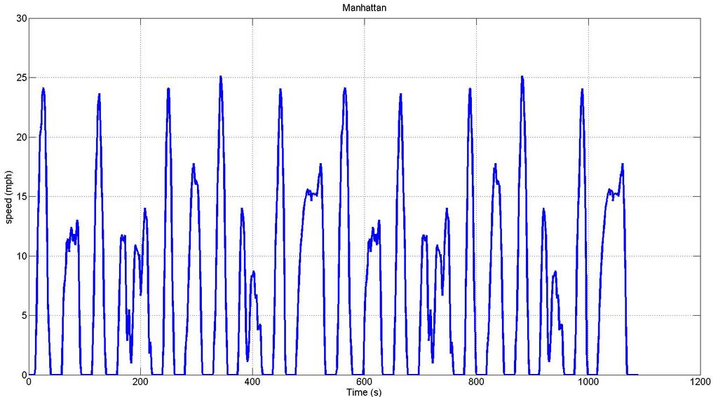
76 75